Parametric Equations (Part 2)

(This page is Part 2. Click here for Part 1.)

Constructing a Parametric Curve with Desired Properties

Suppose we want to travel between two fixed points, $\,P_1(x_1,y_1)\,$ and $\,P_2(x_2,y_2)\,,$ in a fixed time. More specifically, we want to be at $\,P_1\,$ at time $\,t_1\,,$ and at $\,P_2\,$ at time $\,t_2\,$ (with $\,t_1\ne t_2\,$).

Of course, there are many different ways to travel between two points! The simplest solution is a straight line path between the two.

Using function notation, we want:

$$ \begin{align} \cssId{s6}{x(t_1) = x_1}\cr \cssId{s7}{x(t_2) = x_2}\cr \cssId{s8}{y(t_1) = y_1}\cr \cssId{s9}{y(t_2) = y_2} \end{align} $$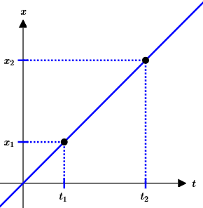

getting a straight line parametric curve between two points

Using point-slope form in the $tx$-plane, we get:

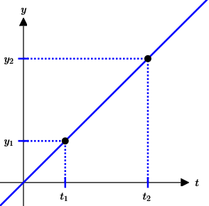
$$ \begin{gather} \cssId{s11}{x(t) - x_1 = \frac{x_2-x_1}{t_2-t_1}(t - t_1)}\cr\cr \cssId{s12}{x(t) = x_1 + \frac{x_2-x_1}{t_2-t_1}(t - t_1)}\tag{9a} \end{gather} $$

Similarly,

$$ \cssId{s14}{y(t) = y_1 + \frac{y_2-y_1}{t_2-t_1}(t - t_1)}\tag{9b} $$

Equations (9a) and (9b) are the desired parametric equations. Together, they give a line through points $\,P_1(x_1,y_1)\,$ and $\,P_2(x_2,y_2)\,$ satisfying:

at time $\,t_1\,$ you're at $\,P_1\,$
at time $\,t_2\,$ you're at $\,P_2\,$

Example

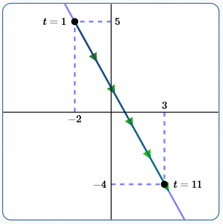
a straight line parametric curve between two given points

The line above is at:

$\,P_1(-2,5)\,$ at time $\,t = 1$
$\,P_2(3,-4)\,$ at time $\,t = 11$

It was generated by substituting the following values into equations (9a) and (9b):

$$ \begin{gather} x_1 = -2\cr y_1 = 5\cr t_1 = 1\cr\cr x_2 = 3\cr y_2 = -4\cr t_2 = 11 \end{gather} $$

giving

$$ \begin{gather} \cssId{s26}{x(t) = -2 + \frac{1}{2}(t - 1)}\cr\cr \cssId{s27}{y(t) = 5 + \frac{-9}{10}(t - 1)} \end{gather} $$

Measuring $\,t\,$ in (say) seconds, each arrow represents the part of the curve traced in two seconds.

Eliminating the Parameter: Going from a Parametric Curve to $\,y = f(x)\,$ (When Possible)

Suppose a parametric curve passes a vertical line test: like examples 1, 2, 3, 4, 6, 9ab (but not 5, 7, 8). Then, you may be able to get a description of the curve in the form ‘$\,y = f(x)\,$’.

In the ‘$\,y = f(x)\,$’ form, you lose information about how the curve is traced out, but this single-equation form may be easier to work with for some applications.

When we want to emphasize that an $x$-value depends on (say) $\,t\,,$ we can write ‘$\,x = x(t)\,$’. Read this aloud as: ‘$\,x\,$ equals $\,x\,$ of $\,t\,$’, meaning that the $x$-value is a function of $\,t\,.$

In going from a pair of parametric equations ‘$\,x = x(t)\,$ and $\,y = y(t)\,$’ to a single equation ‘$\,y = f(x)\,$’, the parameter $\,t\,$ has been eliminated—it is gone! Therefore, this process is typically referred to as ‘eliminating the parameter’.

The process of eliminating the parameter is often used to help identify the graph of parametric equations. It may be easier to recognize a curve in ‘$\,y = f(x)\,$’ form than in parametric equation form.

Example: Eliminating the Parameter in Examples 1–4

Procedure:

Drop function notation: that is, write $\,x(t)\,$ as simply $\,x\,$; write $\,y(t)\,$ as simply $\,y\,.$
Solve for $\,t\,$ in a simplest equation; substitute this expression for $\,t\,$ into the remaining equation.

Note:

In examples 1–4, the equation for $\,x(t)\,$ is simplest to solve for $\,t\,.$
Upon eliminating the parameter, all four curves give $\,y = x^2\,.$

Example (1)

$$ \begin{gather} \cssId{s54}{x(t) = t\,,\ \ y(t) = t^2}\cr \cssId{s55}{\text{Original parametric equations}}\cr\cr \cssId{s56}{x = t\,,\ \ y = t^2}\cr \cssId{s57}{\text{Drop function notation}}\cr\cr \cssId{s58}{t = x}\cr \cssId{s59}{\text{Solve for $\,t\,$ in simplest equation}}\cr\cr \cssId{s60}{y = t^2 = x^2}\cr \cssId{s61}{\text{Substitute into remaining equation}}\cr\cr \cssId{s62}{y = x^2}\cr \cssId{s63}{\text{($\,y = f(x)\,$ form)}} \end{gather} $$

Example (2)

$$ \begin{gather} \cssId{s65}{x(t) = 2t\,,\ \ y(t) = 4t^2}\cr \cssId{s66}{\text{Original parametric equations}}\cr\cr \cssId{s67}{x = 2t\,,\ \ y = 4t^2}\cr \cssId{s68}{\text{Drop function notation}}\cr\cr \cssId{s69}{t = \frac x2}\cr \cssId{s70}{\text{Solve for $\,t\,$ in simplest equation}}\cr\cr \cssId{s71}{y = 4t^2 = 4\bigl(\frac x2\bigl)^2 = \frac{4x^2}{4} = x^2}\cr \cssId{s72}{\text{Substitute into remaining equation}}\cr\cr \cssId{s73}{y = x^2}\cr \cssId{s74}{\text{($\,y = f(x)\,$ form)}} \end{gather} $$

Example (3)

$$ \begin{gather} \cssId{s76}{x(t) = \frac 12t\,,\ \ y(t) = \frac{t^2}4}\cr \cssId{s77}{\text{Original parametric equations}}\cr\cr \cssId{s78}{x = \frac 12t\,,\ \ y = \frac{t^2}4}\cr \cssId{s79}{\text{Drop function notation}}\cr\cr \cssId{s80}{t = 2x}\cr \cssId{s81}{\text{Solve for $\,t\,$ in simplest equation}}\cr\cr \cssId{s82}{y = \frac{t^2}4 = \frac{(2x)^2}4 = \frac{4x^2}4 = x^2}\cr \cssId{s83}{\text{Substitute into remaining equation}}\cr\cr \cssId{s84}{y = x^2}\cr \cssId{s85}{\text{($\,y = f(x)\,$ form)}} \end{gather} $$

Example (4)

$$ \begin{gather} \cssId{s87}{x(t) = -t\,,\ \ y(t) = t^2}\cr \cssId{s88}{\text{Original parametric equations}}\cr\cr \cssId{s89}{x = -t\,,\ \ y = t^2}\cr \cssId{s90}{\text{Drop function notation}}\cr\cr \cssId{s91}{t = -x}\cr \cssId{s92}{\text{Solve for $\,t\,$ in simplest equation}}\cr\cr \cssId{s93}{y = t^2 = (-x)^2 = x^2}\cr \cssId{s94}{\text{Substitute into remaining equation}}\cr\cr \cssId{s95}{y = x^2}\cr \cssId{s96}{\text{($\,y = f(x)\,$ form)}} \end{gather} $$

Example: Eliminating the Parameter in 9ab

To eliminate the parameter, you don't have to solve for (just) $\,t\,.$

As illustrated in this example, it's sometimes easier to solve for a different expression (involving $\,t\,$) that appears in both $\,x(t)\,$ and $\,y(t)\,.$ Here, we solve for $\,t - t_1\,$:

$$ \begin{gather} x(t) = x_1 + \frac{x_2-x_1}{t_2-t_1}(t - t_1)\cr\cr y(t) = y_1 + \frac{y_2-y_1}{t_2-t_1}(t - t_1)\cr\cr \cssId{s103}{\text{Original parametric equations}} \end{gather} $$

$$ \begin{gather} x = x_1 + \frac{x_2-x_1}{t_2-t_1}(t - t_1)\cr\cr y = y_1 + \frac{y_2-y_1}{t_2-t_1}(t - t_1)\cr\cr \cssId{s105}{\text{Drop function notation}} \end{gather} $$

$$ \begin{gather} \cssId{s106}{t-t_1 = \frac{(x-x_1)(t_2-t_1)}{x_2-x_1}}\cr\cr \cssId{s107}{\text{Solve for $\,t-t_1\,$ in the equation for $\,x\,$}} \end{gather} $$

$$ \begin{gather} \cssId{s108}{y = y_1 + \frac{y_2-y_1}{t_2-t_1}\cdot\frac{(x-x_1)(t_2-t_1)}{x_2-x_1}}\cr\cr \cssId{s109}{\text{Substitute into remaining equation}} \end{gather} $$

$$ \begin{gather} \cssId{s110}{y = y_1 + \frac{y_2-y_1}{x_2-x_1}(x - x_1)}\cr\cr \cssId{s111}{\Large\substack{\text{Cancel; re-arrange factors;}\\ \text{this is $\,y = f(x)\,$ form}}} \end{gather} $$

$$ \begin{gather} \cssId{s112}{y - y_1 = \frac{y_2-y_1}{x_2-x_1}(x - x_1)}\cr\cr \cssId{s113}{\Large\substack{\text{Point-slope form for line}\\ \text{through $\,(x_1,y_1)\,$ and $\,(x_2,y_2)\,$}}} \end{gather} $$

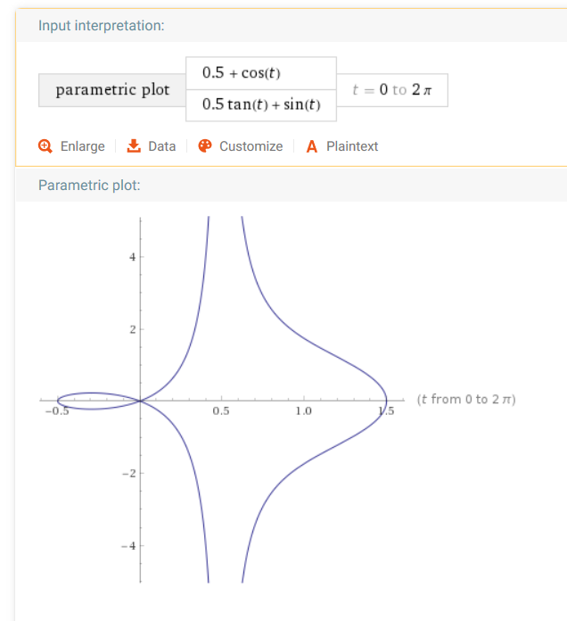
Parametric Equations at WolframAlpha

Hop up to WolframAlpha and type in (say):

parametric plot (0.5 + cos(t) , 0.5*tan(t) + sin(t)), t=0 to 2pi

(You can cut-and-paste.) Voila! How easy is that?

Congratulations on finishing Precalculus!! Next up—Calculus!