Exponential Growth and Decay: Introduction

Exponential functions are of the form $\,y = b^t\,$ for $\,b \gt 0\,$ and $\,b\ne 1\,.$

For $\,b \gt 1\,$ they are increasing, and are called exponential growth functions.

For $\,0 \lt b \lt 1\,$ they are decreasing, and are called exponential decay functions.

All exponential functions share common behavior: when the input changes by a fixed amount, the output gets multiplied by a scaling factor.

It might be that every hour (the fixed input change), something doubles (gets multiplied by $\,2\,$). Or, it might be that every three seconds (the fixed input change), something gets halved (multiplied by $\,\frac 12\,$).

In general, increasing exponential functions get big fast, and decreasing exponential functions get small fast.

A typical exponential growth/decay problem often has this flavor:

A population has a given initial size. Later, it is bigger (or smaller). Assuming exponential behavior, what is its size at some future time?

There are a couple things that can make exponential growth/decay problems seem tricky.

First of all, a ‘basic’ exponential function may need to be generalized, using both vertical and horizontal stretches.

Secondly, the generalized exponential functions go by lots of different names.

You might see a problem solved in different ways, and wonder ‘which is right’. They're all right! Different people choose different names to work with! These issues are discussed in this section.

Choose $\,t = 0\,$

For exponential growth/decay problems, we call the input $\,t\,$ (for ‘time’) instead of $\,x\,.$ Populations change with time; populations are a function of time. The notation $\,P(t)\,$ denotes the size of a population at time $\,t\,.$

You always have an initial choice to make—what you call ‘time zero’—the ‘origin’ for time. Some people choose the earliest time when a population is known to correspond to $\,t = 0\,.$ It doesn't matter, as long as you are consistent throughout the entire problem.

Suppose $\,t=0\,$ is chosen to correspond to time $\,Y\,$ (think ‘year’):

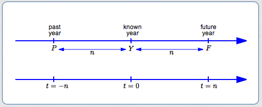
Then, for $\,n \gt 0\,$:

• $\,t = n\,$ corresponds to $\,F = Y + n\,$ (future)
• $\,t = -n\,$ corresponds to $\,P = Y - n\,$ (past)

Going the other direction, for $\,F \gt Y \gt P\,$:

• a future $\,F\,$ corresponds to positive time $\,t = F - Y\,$
• a past $\,P\,$ corresponds to negative time $\,t = P - Y\,$

Generalizing $\,y = b^t\,$ to Handle Typical Exponential Growth/Decay Problems

Pick any allowable value of $\,b\,.$ The sketches below assume $\,b \gt 1\,,$ but the discussion holds for any $\,b \gt 0\,,$ $\,b\ne 1\,.$

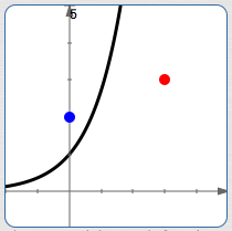
A typical exponential function, $\,y = b^t\,.$ It may not have the correct initial size (the blue point). It may not have the correct second known size (the red point).

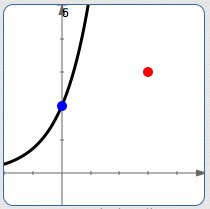
Do a vertical scaling to get the correct initial size:
$y = P_{0}\,b^t$

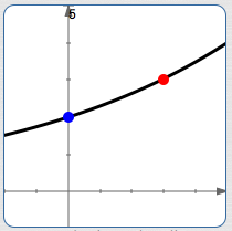
Do a horizontal scaling to get the correct second known size:
$y = P_{0}\,b^{st}$

The exponential function $\,P(t) = b^t\,$ is too restrictive for exponential growth/decay problems. We need to allow for any initial population size. (The ‘initial population’ is the size at $\,t = 0\,.$ ) However, $\,P(0) = b^0 \,\overset{\text{always}}{=}\, 1\,.$ We don't always have an initial population of size $\,1\,$!

To solve this problem, do a vertical scaling of the basic exponential function, giving $\,P(t) = P_{0}\,b^t\,.$ With this generalization, $$ \cssId{s56}{P(0) = P_{0}\, b^0 = P_{0}(1) = P_{0}} $$ so $\,P_{0}\,$ is the desired initial population size. (You can read ‘$\,P_{0}\,$’ as ‘$\,P\,$ sub zero’ or ‘$\,P\,$ naught’.)

We also need the curve to pass through a second point, which describes the population at some known future or past time. A horizontal scaling accomplishes this:   $\,P(t) = P_{0}\, b^{st}\,$

Checking That the Generalized Exponential Function Still Behaves As Expected

It's worthwhile to check that the generalized exponential function, $\,P(t) = P_{0}\, b^{st}\,,$ still has the property mentioned above: when the input changes by a fixed amount, the output gets multiplied by a scaling factor.

In this case, the scaling factor is $\,b^{s\Delta t}\,,$ which depends on three things:

• the base of the exponential function ($\,b\,$)
• the horizontal scaling factor ($\,s\,$)
• how much the inputs are changing by ($\,\Delta t\,$)

Any Generalized Exponential Function Can Be Written With Any Allowable Base

Let $\,b\,,$ $\,k\,$ and $\,s\,$ be the current base, vertical scaling factor, and horizontal scaling factor for a generalized exponential function:

You've decided you don't want base $\,b\,.$ You want a different base $\,B\,$ instead. This can be easily done!

Let $\,y = KB^{St}\,$ denote the new function, with the desired base. Notice that we're using lowercase letters for the old function ($\,b\,,$ $\,k\,,$ $\,s\,$), and uppercase letters for the new function ($\,B\,,$ $\,K\,,$ $\,S\,$).

• We want $\,kb^{st} = KB^{St}\,$ to be true for all values of $\,t\,.$
• In particular, it must be true when $\,t = 0\,.$ Substituting $\,0\,$ for $\,t\,$ gives $\,kb^0 = KB^0\,,$ so that $\,k = K\,.$ The vertical scaling factor stays the same!
• Now we have $\,kb^{st} = kB^{St}\,.$ Divide both sides by $\,k\,,$ giving $\,b^{st} = B^{St}\,.$
• To get to the exponents, take logs of both sides. Any log will do, so choose the natural logarithm: $\,\ln b^{st} = \ln B^{St}$
• Bring down the exponents: $\,st \ln b = St\ln B$
• Divide both sides by $\,t\,$: $\,s\ln b = S\ln B$
• Solve for $\,S\,$: $\,\displaystyle S = s\cdot\frac{\ln b}{\ln B}$

Here's a quick example to show how easy it is!

Initial function:
$\,y = 10\cdot 5^{3t}$
($\,k = 10\,,$ $\,b = 5\,,$ $\,s = 3\,$)

New desired base: $\,7$
($\,B = 7\,$)

The $\,10\,$ stays the same ($\,K = k\,$).

The new horizontal scaling factor is:

The new function is therefore: $$y = K\cdot B^{St} = 10\cdot 7^{3t(\ln 5)/(\ln 7)}$$

Don't take my word for it! Hop up to wolframalpha.com and cut-and-paste:

plot y = 10 * 5^{3t}, y = 10 * 7^{3t ln(5)/ln(7)}

You'll only see one curve, because they're exactly the same!

So, any base can be written as any other base. Exponential functions have lots of different names!

The point is this:  when solving exponential growth/decay problems, you can use any (allowable) base that you want. Having said this, though, there is a strongly-favored base that is usually used $\ldots$

Since Any Base Can Be Used, Most People Use Base $\,\text{e}\,$

Since any base can be used when solving exponential growth/decay problems, most people use base $\,\text{e}\,.$ Why? Why would someone want to use an irrational number as a base, instead of a ‘simple’ number like (say) $\,2\,$?

The answer is that the exponential function with base $\,\text{e}\,$ has calculus properties that make it easier to work with than any other exponential function. Also, when the base is $\,\text{e}\,,$ the horizontal scaling constant takes on special significance, and is given a special name—the relative growth rate. More on this in the next section!