2.4 Nonlinear Least Squares Approximation
A Linearizing Technique and Gradient Methods
Let $\,\{(t_i,y_i)\}_{i=1}^N\,$ be a given data set. Consider the following minimization problem:
Find a sinusoid that best approximates the data, in the least-squares sense. That is, find real constants $\,A\ne 0\,,$ $\,\phi\,,$ and $\,\omega\ne 0\,$ so that the function $\,f\,$ given by
$$ f(t) = A\sin(\omega t + \phi) $$minimizes the sum of the squared errors between $\,f(t_i)\,$ and $\,y_i\,$:
$$ \begin{align} SSE &:= \sum_{i=1}^N \bigl( y_i - f(t_i) \bigr)^2\cr &= \sum_{i=1}^N \bigl( y_i - A\sin(\omega t_i + \phi) \bigr)^2 \end{align} $$This problem differs from the least-squares problem considered in Section 2.2, in that the parameters to be ‘adjusted’ ($\,A\,,$ $\,\phi\,,$ and $\,\omega\,$) do not all appear linearly in the formula for the approximate $\,f\,.$ (This notion of linear dependence on a parameter is made precise below.)
Consequently, the resulting problem is called nonlinear least-squares approximation, and is exceedingly more difficult to solve, because it does not lend itself to exact solution by matrix methods.
Indeed, nonlinear least-squares problems must generally be solved by iterative techniques. Nonlinear least-squares approximation is the subject of this section.
First, a definition:
Suppose $\,f\,$ is a function that depends on time, a fixed parameter $\,b\,,$ and possibly other parameters. This dependence is denoted by $\,f = f(t,b,x)\,,$ where $\,x\,$ represents all other parameters.
The function $\,f\,$ is said to be linear with respect to the parameter $\,b\,$ if and only if the function $\,f\,$ has the form
$$ f(t,b,x) = b\cdot f_1(t,x) + f_2(t,x) $$for functions $\,f_1\,$ and $\,f_2\,$ that may depend on $\,t\,$ and $\,x\,,$ but not on $\,b\,.$
This definition is generalized in the obvious way. For example, a function $\,f = f(t,b_1,b_2,x)\,$ is linear with respect to the parameters $\,b_1\,$ and $\,b_2\,$ if and only if $\,f\,$ has the form
$$ f(t,b_1,b_2,x) = b_1\cdot f_1(t,x) + b_2\cdot f_2(t,x) + f_3(t,x) $$for functions $\,f_1\,,$ $\,f_2\,,$ and $\,f_3\,$ that may depend on $\,t\,$ and $\,x\,,$ but not on $\,b_1\,$ and $\,b_2\,.$
Example
The function $\,f(t,A,\phi,\omega) = A\sin(\omega t + \phi)\,$ is linear with respect to the parameter $\,A\,,$ but not linear with respect to $\,\phi\,$ or $\,\omega\,.$
If $\,f\,$ depends linearly on a parameter $\,b\,,$ then $\,\frac{\partial SSE}{\partial b}$ also depends linearly on $\,b\,,$ as follows:
$$ \begin{align} SSE &= \sum_{i=1}^N \bigl( y_i - b\cdot f_1(t_i,x) - f_2(t_i,x) \bigr)^2\,;\cr\cr \frac{\partial SSE}{\partial b} &= \sum_{i=1}^N\ 2 \bigl( y_i - b\cdot f_1(t_i,x)\cr &\qquad\qquad - f_2(t_i,x) \bigr) \cdot \bigl( -f_1(t_i,x) \bigr)\cr\cr &= b\cdot\sum_{i=1}^N\,2\bigl(f_1(t_i,x)\bigr)^2\cr &\qquad - 2\sum_{i=1}^N y_if_1(t_i,x) - f_1(t_i,x)f_2(t_i,x) \end{align} $$Similarly, if $\,f\,$ depends linearly on parameters $\,b_1,\ldots,b_m\,,$ then so do $\,\frac{\partial SSE}{\partial b_i}\,$ for all $\,i = 1,\ldots,m\,.$ Consequently, as seen in Section 2.2, matrix methods can be used to find parameters that make the partials equal to zero.
Unfortunately, when $\,f\,$ does NOT depend linearly on a parameter $\,b\,,$ the situation is considerably more difficult, as illustrated next:
Example
Let $\,f(t) = A\sin(\omega t + \phi)\,,$ so that, in particular, $\,f\,$ does not depend linearly on $\,\omega\,.$ In this case, differentiation of
$$ SSE = \sum_{i=1}^N \bigl( y_i - A\sin(\omega t_i + \phi) \bigr)^2 $$with respect to $\,\omega\,$ yields:
$$ \begin{align} \frac{\partial SSE}{\partial\omega} &= \sum_{i=1}^N\ 2 \bigl( y_i - A\sin(\omega t_i + \phi) \bigr)\cr &\qquad\qquad \cdot \bigl( -At_i\cos(\omega t_i + \phi) \bigr) \end{align} $$Even if $\,A\,$ and $\,\phi\,$ are held constant, the equation $\,\frac{\partial SSE}{\partial\omega} = 0\,$ is not easy to solve for $\,\omega\,.$
Since a linear dependence on parameters is desirable, it is reasonable to try and replace the class of approximating functions,
$$ \begin{align} {\cal F} &= \{ f\ |\ f(t) = A\sin(\omega t + \phi)\,,\cr &\qquad A\ne 0\,, \phi\in\Bbb R\,, \omega \ne 0 \} \end{align} \tag{1} $$with another class $\,\overset{\sim }{\cal F}\,,$ that satisfies the following properties:
- $\cal F = \overset{\sim }{\cal F}\,,$ and
- The new class $\,\overset{\sim }{\cal F}\,$ involves functions that have more linear dependence on the approximating parameters than the original class.
If it is possible to find such a class $\,\overset{\sim }{\cal F}\,,$ then the process of replacing $\,\cal F\,$ by $\,\overset{\sim }{\cal F}\,$ is called a linearizing technique.
Example
For example, the next lemma shows that the set
$$ \begin{align} \overset{\sim}{\cal F} &:= \{ f\ |\ f(t) = C\sin\omega t + D\cos\omega t\,,\cr &\qquad \omega\ne 0\,, C\ \text{ and } D \text{ not both zero} \} \end{align} $$is equal to the set $\,\cal F\,$ given in ($1$). Thus, any function representable in the form $\,A\sin(\omega t + \phi)\,$ is also representable in the form $\,C\sin\omega t + D\cos\omega t\,,$ and vice versa.
Both classes $\,\cal F\,$ and $\,\overset{\sim}{\cal F}\,$ involve three parameters: $\,\cal F\,$ involves $\,A\,,$ $\,\phi\,$ and $\,\omega\,$; and $\,\overset{\sim}{\cal F}\,$ involves $\,C\,,$ $\,D\,$ and $\,\omega\,.$
However, a function $\,f(t) = C\sin\omega t + D\cos\omega t\,$ from $\,\overset{\sim}{\cal F}\,$ depends linearly on both $\,C\,$ and $\,D\,,$ whereas $\,f(t) = A\sin(\omega t + \phi)\,$ only depends linearly on $\,A\,.$ Thus, the class $\,\overset{\sim}{\cal F}\,$ is more desirable.
Let $\,\cal F\,$ and $\,\overset{\sim }{\cal F}\,$ be classes of functions of one variable, defined by:
$$ \begin{align} {\cal F} &= \{ f\ |\ f(t) = A\sin(\omega t + \phi)\,,\cr &\qquad A\ne 0\,, \phi\in\Bbb R\,, \omega \ne 0 \} \end{align} $$ $$ \text{and} $$ $$ \begin{align} \overset{\sim}{\cal F} &:= \{ f\ |\ f(t) = C\sin\omega t + D\cos\omega t\,,\cr &\qquad \omega\ne 0\,, C\ \text{ and } D \text{ not both zero} \} \end{align} $$Then, $\,\cal F = \overset{\sim}{\cal F}\,.$
Proof
Let $\,f\in \cal F\,.$ For all $\,t\,,$ $\,A\,,$ $\,\phi\,$ and $\,\omega\,$:
$$ \begin{align} f(t) &= A\sin(\omega t + \phi)\cr\cr &= A(\sin\omega t\cos\phi + \cos\omega t\sin\phi)\cr\cr &= \overbrace{(A\cos\phi)}^{C}\sin\omega t + \overbrace{(A\sin\phi)}^{D}\cos\omega t \tag{*} \end{align} $$Define $\, C := A\cos\phi\,$ and $\,D := A\sin\phi\,.$ Since $\,f\in\cal F\,,$ one has $\,A\ne 0\,.$ Therefore, the only way that both $\,C\,$ and $\,D\,$ can equal zero is if $\,\cos\phi = \sin\phi = 0\,,$ which is impossible. Thus, $\,f\in \overset{\sim}{\cal F}\,.$
Now, let $\,f\in\overset{\sim}{\cal F}\,,$ so that $\,f(t) = C\sin\omega t + D\cos \omega t\,$ for $\,\omega\ne 0\,,$ for numbers $\,C\,$ and $\,D\,$ that are not both zero. It may be useful to refer to the flow chart below while reading the remainder of the proof.
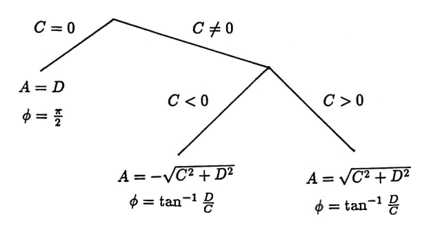
If $\,C = 0\,,$ then $\,D\ne 0\,.$ In this case:
$$ \begin{align} &C\sin\omega t + D\cos\omega t\cr &\quad = D\cos\omega t\cr &\quad = D\sin(\omega t + \frac\pi 2) \end{align} $$Take $\,A := D\,,$ and $\,\phi = \frac\pi 2\,$ to see that $\,f\in\cal F\,.$
Now, let $\,C\ne 0\,.$ If there exist constants $\,A\ne 0\,$ and $\,\phi\,$ for which $\,C = A\cos\phi\,$ and $\,D = A\sin\phi\,,$ then $\,A\,$ and $\,\phi\,$ must satisfy certain requirements, as follows:
Since $\,C\ne 0\,,$ it follows that $\,\cos\phi \ne 0\,.$ Thus:
$$ \frac DC = \frac{A\sin\phi}{A\cos\phi} = \tan\phi $$There are an infinite number of choices for $\,\phi\,$ that satisfy this requirement. Choose $\,\phi := \tan^{-1}\frac DC\,,$ where $\,\tan^{-1}\,$ denotes the arctangent function, defined by:
$$ \begin{gather} y = \tan^{-1}x\cr \iff\cr \bigl( \tan y = x\ \text{ and }\ y\in (-\frac\pi 2,\frac\pi 2)\, \bigr) \end{gather} $$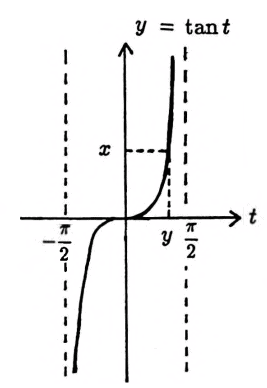
Also note that
$$ \begin{align} &C^2 + D^2\cr &\quad = (A\cos\phi)^2 + (A\sin\phi)^2\cr &\quad = A^2\,, \end{align} $$so that $\,A\,$ must equal either $\,\sqrt{C^2 + D^2}\,$ or $\,-\sqrt{C^2 + D^2}\,.$
The table below gives the correct formulas for
$$ \cos\bigl(\tan^{-1}\frac DC\bigr) \ \ \text{and}\ \ \sin\bigl(\tan^{-1}\frac DC\bigr)\ , $$for all possible sign choices of C and D. In this table:
$$ K := \sqrt{C^2 + D^2} $$| $D$ | $C$ | $\sin\bigl(\tan^{-1}\frac DC\bigr)$ | $\cos\bigl(\tan^{-1}\frac DC\bigr)$ |
| $+$ | $+$ | $\frac DK$ | $\frac CK$ |
| $+$ | $-$ | $-\frac DK$ | $-\frac CK$ |
| $-$ | $+$ | $\frac DK$ | $\frac CK$ |
| $-$ | $-$ | $-\frac DK$ | $-\frac CK$ |
If $\,C \gt 0\,,$ then take $\,A := \sqrt{C^2 + D^2}\,.$ Using (*):
$$ \begin{align} &A\sin(\omega t + \phi)\cr\ &\quad = \sqrt{C^2 + D^2}\,\cos\bigl(\tan^{-1}\frac DC\bigr)\sin\omega t\cr &\qquad + \sqrt{C^2+D^2}\,\sin\bigl(\tan^{-1}\frac DC\bigr)\cos\omega t\cr &= \sqrt{C^2 + D^2}\,\frac{C}{\sqrt{C^2+D^2}}\,\sin\omega t\cr &\qquad + \sqrt{C^2+D^2}\,\frac{D}{\sqrt{C^2+D^2}}\,\cos\omega t\cr &\quad = C\sin\omega t + D\cos\omega t \end{align} $$If $\,C \lt 0\,,$ take $\,A := -\sqrt{C^2 + D^2}\,.$ Then:
$$ \begin{align} &A\sin(\omega t + \phi)\cr\ &\quad = -\sqrt{C^2 + D^2}\,\cos\bigl(\tan^{-1}\frac DC\bigr)\sin\omega t\cr &\qquad - \sqrt{C^2+D^2}\,\sin\bigl(\tan^{-1}\frac DC\bigr)\cos\omega t\cr &= -\sqrt{C^2 + D^2}\,\frac{-C}{\sqrt{C^2+D^2}}\,\sin\omega t\cr &\qquad - \sqrt{C^2+D^2}\,\frac{-D}{\sqrt{C^2+D^2}}\,\cos\omega t\cr &\quad = C\sin\omega t + D\cos\omega t \end{align} $$In both cases, it has been shown that $\,f\in\cal F\,.$ $\blacksquare$
The following iterative approach can be used to find a choice of parameters $\,C\,,$ $\,D\,$ and $\,\omega\,$ so that the function $\,f(t) = C\sin\omega t + D \cos\omega t\,$ best approximates the data, in the least-squares sense. Observe that, once a value of $\,\omega\,$ is fixed, the remaining problem is just linear least-squares approximation, treated in Section $2.2\,.$
- Estimate a value of $\,\omega\,,$ based perhaps on initial data analysis.
- Use the methods from Section $2.2\,$ to find optimal parameters $\,C\,$ and $\,D\,$ corresponding to $\,\omega\,.$
- Compute the sum of squared errors, $\,SSE(C,D,\omega)\,,$ corresponding to $\,C\,,$ $\,D\,$ and $\,\omega\,.$
- Try to decrease $\,SSE\,$ by adjusting $\,\omega\,,$ and repeating the process.
One algorithm for ‘adjusting’ $\,\omega\,$ is based on the following result from multivariable calculus:
Let $\,h\,$ be a function from $\,\Bbb R^m\,$ into $\,\Bbb R\,,$ and let $\,\boldsymbol{\rm x} = (x_1,\ldots,x_m)\,$ be an element of $\,\Bbb R^m\,.$
If $\,h\,$ has continuous first partials in a neighborhood of $\,\boldsymbol{\rm x}\,,$ then the function $\,\triangledown h\ :\ \Bbb R^m\rightarrow\Bbb R^m\,$ defined by
$$ \triangledown h(x_1,\ldots,x_m) := \bigl( \frac{\partial h}{\partial x_1}(\boldsymbol{\rm x}),\ldots, \frac{\partial h}{\partial x_m}(\boldsymbol{\rm x}) \bigr) $$has the following property:
At $\,\boldsymbol{\rm x}\,,$ the function $\,h\,$ increases most rapidly in the direction of the vector $\,\triangledown h(\boldsymbol{\rm x})\,$ (the rate of change is then $\,\|\triangledown h(\boldsymbol{\rm x})\|\,$), and decreases most rapidly in the direction of $\,-\triangledown h(\boldsymbol{\rm x})\,$ (the rate of change is then $\,-\|\triangledown h(\boldsymbol{\rm x})\|\,$).
The function $\,\triangledown h\,$ is called the gradient of $\,h\,.$
This theorem will be used to ‘adjust’ parameter(s) so that the function $\,SSE\,$ will decrease most rapidly.
- Let $\,\omega\,$ be a current parameter value.
-
Compute $\,\triangledown SSE(\omega)\,.$ One must move in the direction of $\,-\triangledown SSE(\omega)\,$ to decrease $\,SSE\,$ most rapidly. Thus, let $\,\epsilon\,$ be a small positive number, and compute:
$$ \omega_{\text{new}} = \omega - \epsilon\cdot\frac{\triangledown SSE(\omega)}{\|\triangledown SSE(\omega)\|} $$
When $\,\|\triangledown SSE(\omega)\|\,$ is large, the function $\,SSE\,$ is changing rapidly at $\,\omega\,$; when $\,\|\triangledown SSE(\omega)\|\,$ is small, the function $\,SSE\,$ is changing slowly at $\,\omega\,.$
The MATLAB implementation given in this section allows the user to choose the value of $\,\epsilon\,.$ ‘Optimal’ values of $\,\epsilon\,$ will depend on both the function $\,SSE\,,$ and the current value of $\,\omega\,,$ as suggested by the sketches below (where, for convenience, $\,SSE\,$ is a function of one variable only).
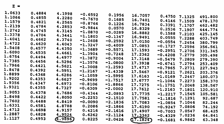
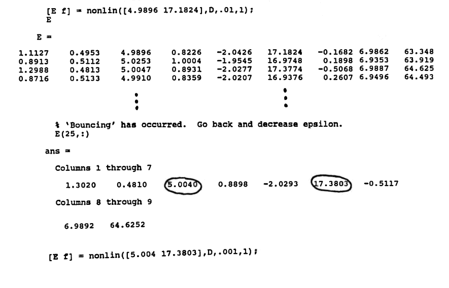
These sketches also illustrate how ‘bouncing’ can occur, and how $\,\omega\,$ can converge to a non-optimal minimum. In general, experience and experimentation by the analyst will play a role in the success of this technique.
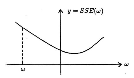
Far away from minimum; large $\,\epsilon\,$ will speed process initially
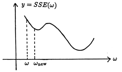
Convergence to ‘wrong’ minimum
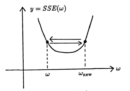
‘Bouncing’
The previous theorem is now applied to a general nonlinear least-squares problem. MATLAB implementation, for a special case of the situation discussed here, will follow.
Let $\,f_1,f_2,\ldots,f_m\,$ be functions that depend on time, and on parameters $\,\boldsymbol{\rm c} := (c_1,\ldots,c_p)\,.$ That is, $\,f_i = f_i(t,\boldsymbol{\rm c})\,$ for $\,i = 1,\ldots,m\,.$ The dependence on any of the inputs may be nonlinear.
Define a function $\,f\,$ that depends on time, the parameters $\,\boldsymbol{\rm c}\,,$ and parameters $\,\boldsymbol{\rm b} = (b_1,\ldots,b_m)\,,$ via:
$$ f(t,c,\boldsymbol{\rm b}) = b_1f_1(t,\boldsymbol{\rm c}) + \cdots + b_mf_m(t,\boldsymbol{\rm c}) $$Thus, $\,f\,$ is linear with respect to the parameters in $\,\boldsymbol{\rm b}\,,$ but not in general with respect to the parameters in $\,\boldsymbol{\rm c}\,.$
Given a data set $\,\{(t_i,y_i)\}_{i=1}^N\,,$ let $\,\boldsymbol{\rm t} = (t_1,\ldots,t_N)\,$ and $\,\boldsymbol{\rm y} = (y_1,\ldots,y_N)\,.$ The sum of the squared errors between $\,f(t_i,\boldsymbol{\rm c},\boldsymbol{\rm b})\,$ and $\,y_i\,$ is
$$ SSE = \sum_{i=1}^N \bigl( y_i - f(t_i,\boldsymbol{\rm c},\boldsymbol{\rm b}) \bigr)^2\,, $$which has partials
$$ \frac{\partial SSE}{\partial c_j} = \sum_{i=1}^N 2\bigl( y_i - f(t_i,\boldsymbol{\rm c},\boldsymbol{\rm b}) \bigr) \bigl( -\frac{\partial f}{\partial c_j}(t_i,\boldsymbol{\rm c},\boldsymbol{\rm b}) \bigr)\,, $$for $\,j = 1,\ldots,p\,.$ Note that:
$$ \begin{align} &\frac{\partial f}{\partial c_j}(t_i,\boldsymbol{\rm c},\boldsymbol{\rm b})\cr &\quad = b_1\frac{\partial f_1}{\partial c_j}(t_i,\boldsymbol{\rm c}) + \cdots + b_m\frac{\partial f_m}{\partial c_j}(t_i,\boldsymbol{\rm c}) \end{align} $$Then, $\,\triangledown SSE = (\frac{\partial SSE}{\partial c_1},\ldots, \frac{\partial SSE}{\partial c_p})\,. $
The algorithm:
- Choose an initial value of $\,(c_1,\ldots,c_p)\,.$
- Use the methods in Section $2.2$ to find corresponding optimal values of $\,(b_1,\ldots,b_m)\,.$
-
Adjust:
$$ (c_1,\ldots,c_p)_{\text{new}} = (c_1,\ldots,c_p) - \epsilon\cdot \frac{\triangledown SSE}{\|\triangledown SSE\|} $$The analyst may need to adjust $\,\epsilon\,$ based on an analysis of the values of $\,SSE\,.$ If $\,SSE\,$ is large, but decreasing slowly, make $\,\epsilon\,$ larger. If $\,SSE\,$ is ‘bouncing’, make $\,\epsilon\,$ smaller.
- Repeat with the new values in $\,\boldsymbol{\rm c}\,.$
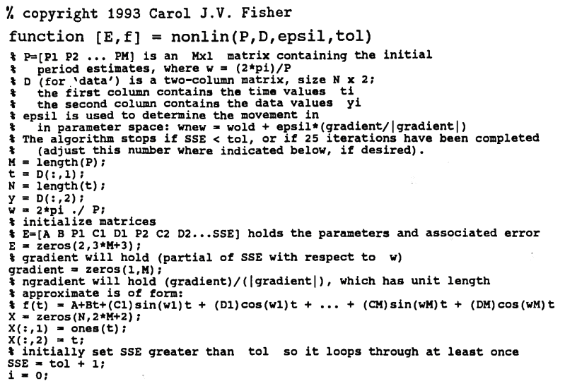
MATLAB IMPLEMENTATION: Nonlinear Least-Squares, Gradient Method
The following MATLAB function uses the gradient method discussed in this section to fit data with a sum of the form:
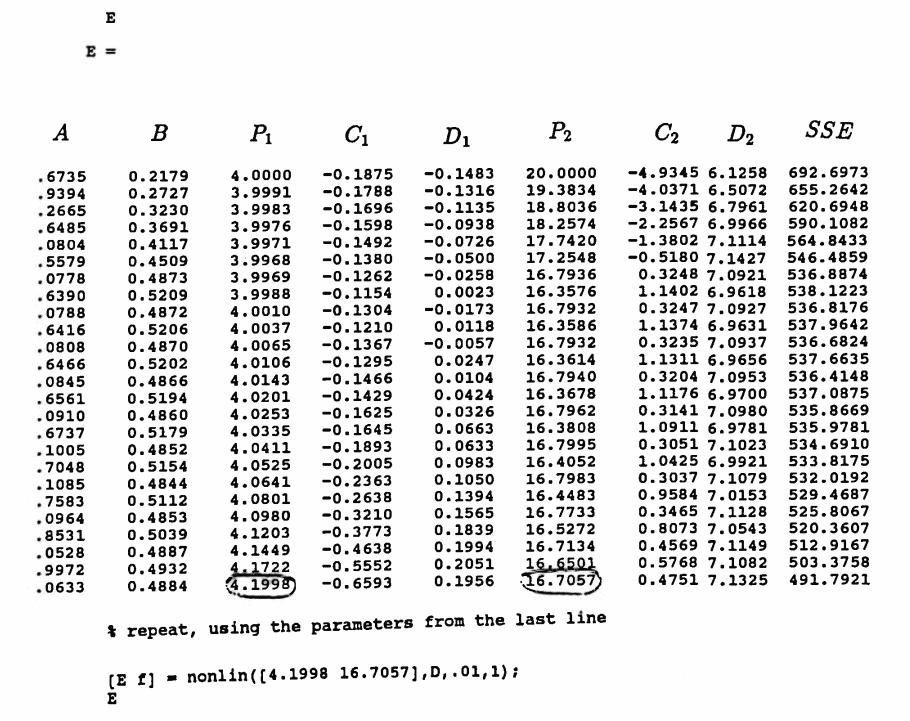
$$ f(t) = A + Bt + \sum_{i=1}^m C_i\sin\omega_i t + D_i\cos\omega_i t $$The fundamental period of $\,\sin\omega_i t\,$ is $\,P_i := \frac{2\pi}{\omega_i}\,.$ To use the function, type:
[E,f] = nonlin(P,D,epsil,tol);
The required inputs are:
- P $\,= [P_1\cdots P_m]\,$ is a matrix containing the initial estimates for the unknown periods. P may be a row or a column matrix.
- D is an $\,N\times 2\,$ matrix containing the data set $\,\{(t_i,y_i)\}_{i=1}^N\,.$ The time values are in the first column; the corresponding data values are in the second column.
-
epsil is used to control the search in parameter space. Indeed:
$$ (P_1,\ldots,P_m)_{\text{new}} = (P_1,\ldots,P_m) - \epsilon \frac{\triangledown SSE}{\|\triangledown SSE\|} $$ - tol is used to help determine when the algorithm stops. The algorithm will stop when either $\,25\,$ iterations have been made, or when $\,SSE \lt \,$ tol .
The function returns the following information:
-
E is a matrix containing each iteration of ‘best’ parameters and the associated error. Each row of E is of the form:
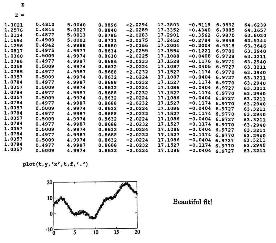
$$ \begin{gather} A\ \ B\ \ P_1\ \ C_1\ \ D_1\ \ P_2\ \ C_2\ \ D_2\cr \cdots\ \ P_m\ \ C_m\ \ D_m\ \ SSE \end{gather} $$ - f contains the values of the approximation to the data, using the parameter values in the last row of the matrix E , and using the time values in t . Then, the command plot(t,y,'x',t,f,'.') can be used to compare the actual data set with the approximate.
The MATLAB function nonlin is given next.
For Octave, the line
X(:,1) = ones(t);
must be changed to:
X(:,1) = ones(size(t));
Also, endfunction must be added as the last line.
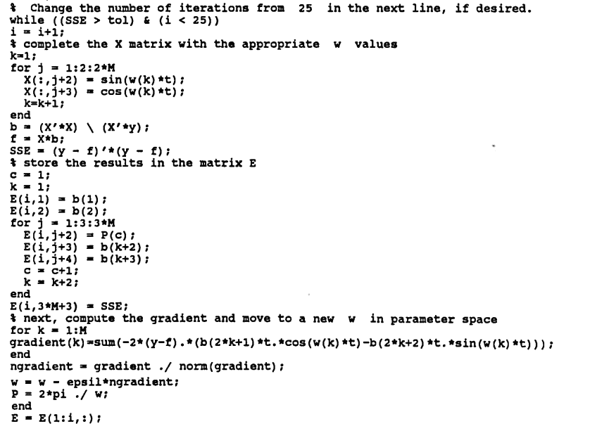
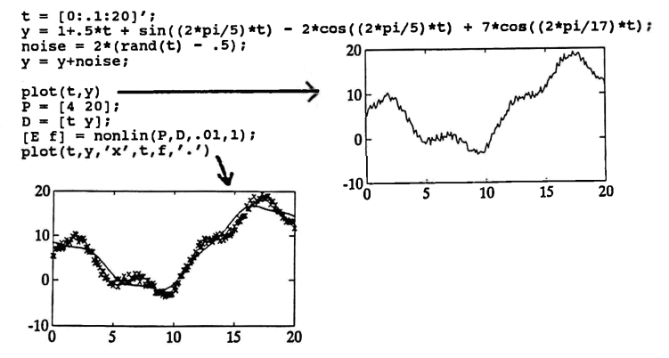
The following diary of an actual MATLAB session illustrates the use of the function nonlin.
For Octave, the line
rand(t)
must be changed to:
rand(size(t))
A Genetic Algorithm
A genetic algorithm is a search technique based on the mechanics of natural selection and genetics. Genetic algorithms may be used whenever there is a real-valued function $\,f\,$ that is to be maximized over a finite set of parameters, $\,S\,$:
$$ \underset{p\,\in\, S}{\text{max}}\ f(p) $$In practice, an infinite parameter space is ‘coded’ to obtain the finite set $\,S\,.$
Genetic algorithms use random choice as a tool to guide the search through the set $\,S\,.$
Notation: Objective Function; Fitness; Parameter Set; Strings
In the context of genetic algorithms, the function $\,f\,$ is called the objective function, and is said to measure the fitness of elements in $\,S\,.$ The set $\,S\,$ is called the parameter set, and its elements are called strings. It will be seen that the elements of $\,S\,$ take the form $\,(p_1,p_2,\ldots,p_m)\,.$
One advantage of genetic algorithms over other optimization methods is that only the objective function $\,f\,$ and set $\,S\,$ are needed for implementation. In particular, there are no continuity or differentiability requirements on the objective function.
Also, genetic algorithms work from a wide selection of points simultaneously (instead of a single point), making it far less likely to hit a ‘wrong’ optimal point.
Genetic algorithms can be particularly useful for determining a ‘starting point’ for the gradient method, when an analyst has no natural candidate.
Here are the basic steps in a simple genetic algorithm:
- (Initialization) An initial population is randomly selected from $\,S\,.$ The objective function $\,f\,$ is used to determine the fitness of each choice from the initial population.
- (Reproduction) A new population is produced, based on the fitness of elements in the original population. Strings with a high level of ‘fitness’ are more likely to appear in the new population.
- (Crossover) This new population is adjusted, by randomly ‘matching up and mixing’ the strings. This information exchange between the ‘fittest’ strings is hoped to produce ‘offspring’ with a fitness greater than their ‘parents’.
-
(Mutation) Mutation is the occasional random alteration of a particular value in a parameter string. In practice, mutation rates are on the order of one alteration per thousand position changes [Gold, p.14].
In the MATLAB implementation discussed in this section, the mutation rate is zero.
The steps above are repeated as necessary. Each new population, formed by reproduction, crossover and (possibly) mutation, is called a generation.
An earlier problem is revisited:
Given a data set $\,\{(t_i,y_i)\}_{i=1}^N\,,$ find parameters $\,A\,,$ $\,B\,,$ $\,C_i\,,$ $\,D_i\,,$ and $\,P_i := \frac{2\pi}{\omega_i}\,$ ($\,i = 1,\ldots,m\,$) so that the function
$$ f(t) = A + Bt + \sum_{i=1}^m C_i\sin\omega_it + D_i\cos\omega_it $$minimizes the sum of the squared errors between $\,f(t_i)\,$ and the data values $\,y_i\,$:
$$ \text{min} \sum_{i=1}^N \ \bigl( f(t_i) - y_i \bigr)^2 $$
A genetic algorithm will be used to search among potential choices for the periods of the sinusoids. For each string $\,(P_1,\ldots,P_m)\,$ in the parameter set, linear least-squares techniques (Section 2.2) will be used to find the corresponding optimal choices for $\,A\,,$ $\,B\,,$ $\,C_i\,$ and $\,D_i\,$ ($\,i = 1,\ldots,m\,$), which are then used to find the mean-square error associated with that string:
$$ \text{error}(P_1,\ldots,P_m) = \sum_{i=1}^N \bigl( f(t_i) - y_i \bigr)^2 $$The objective function will be defined so that strings with minimum error have maximum fitness, and strings with maximum error have minimum fitness.
The reader is now guided through an implementation of a genetic algorithm, using MATLAB. A wealth of additional information can be found in [Gold]. It may be helpful to look ahead to the example while reading through the following discussion of the function genetic.
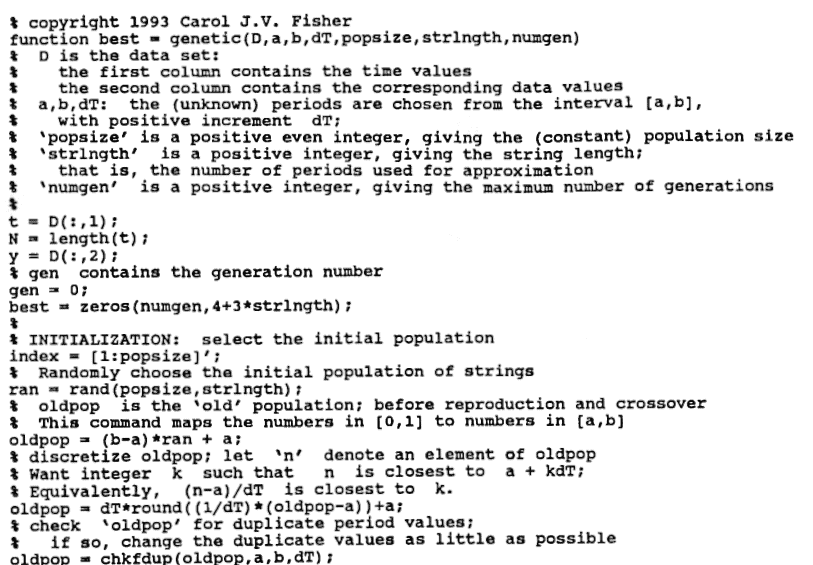
MATLAB Function: genetic
The following MATLAB function uses a genetic algorithm to search for periods $\,P_1,\ldots,P_m\,$ that approximate a solution to (P).
To use the function, type:
best = genetic(D,a,b,dT,popsize,strlngth,numgen);
Important sections of code are analyzed. The entire code is given at the end of this section.
Required Inputs
The required inputs are:
D is an $\,N \times 2\,$ matrix containing the data set $\,\{(t_i,y_i)\}_{i=1}^N\,.$ The first column of D must contain the time values. The second column contains the corresponding data values.
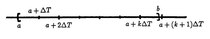
Let $\,a\,$ and $\,b\,$ be positive real numbers with $\,a \lt b\,,$ and let $\,\Delta T\gt 0\,.$ The MATLAB variables a , b and dT correspond, respectively, to $\,a\,,$ $\,b\,$ and $\,\Delta T\,.$
Periods are chosen from the interval $\,[a, b]\,,$ with increment $\,\Delta T\,,$ as follows. Let $\,k\,$ be the greatest nonnegative integer for which $\,a + k\Delta T\le b\,.$ Then, every number in the set
$$\tilde S := \{a, a + \Delta T, a + 2\Delta T,\ldots, a + k\Delta T\}$$is in the interval $\,[a, b]\,.$
Define:
$$ S := \{(P_1,\ldots,P_i,\ldots,P_m)\ |\ P_i\in\tilde S,\ 1\le i\le m\} $$The initial population is chosen from this parameter set $\,S\,.$
popsize is a positive even integer, that gives the size of the population chosen from $\,S\,.$ It is assumed that the population size is constant over all generations.
strlngth gives the length of each string in the parameter set $\,S\,.$ For example, if each string is of the form $\,(P_1,\ldots,P_m)\,,$ then strlngth = m .
numgen gives the number of generations of the genetic algorithm to be implemented.
Output From the Function
The function scrolls information about each generation as it is running. This information is described later on.
The function returns a matrix best that contains the best string of periods, and related information, from each generation of the genetic algorithm. If two strings have equal fitness, then the first such string is returned in best .
Each row of best is of the form:
(generation #) (best string of periods) (error)
$A$ $B$ $C_1$ $D_1$
$C_2$ $D_2$ $\cdots$
$C_m$ $D_m$
Initialization
(INITIALIZATION) The genetic algorithm begins with a random selection of the initial population from the parameter set $\,S\,$.
Each line below is numbered for easy reference in the explanations that follow.
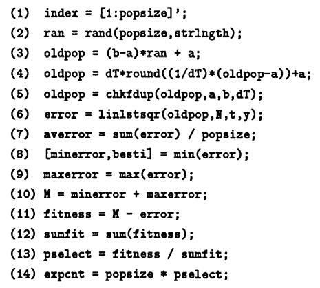
$(1)$ The column vector index is used to number the strings in each population, for easy reference.
$(2)$ The command rand(popsize,strlngth) creates a matrix of size popsize x strlngth with entries randomly chosen (using a uniform distribution) from the interval $\,[0,1]\,.$
$(3)$ The entries in ran are mapped to entries in the interval $\,[a, b]\,,$ via the mapping given below. The resulting matrix is named oldpop , for ‘old population’.
![entries in ran are mapped to [a,b]](graphics/S2_4Img15.png)
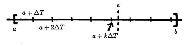
$(4)$ Each entry in oldpop must be replaced by a best approximation from the allowable parameter set, $\,S\,.$ Let $\,e\,$ denote an entry in oldpop . A nonnegative integer $\,k\,$ is sought, so that $\,e\,$ is closest to $\,a + k\Delta T\,.$ Since $\,\Delta T \gt 0\,,$ one has:
$$ \begin{align} &|e - (a+k\Delta T)|\cr\cr &\quad = \left| \Delta T\bigl( \frac{e}{\Delta T} - \frac{a}{\Delta T} - k \bigr) \right|\cr\cr &\quad = \Delta T \left| \frac{e-a}{\Delta T} - k \right| \end{align} $$Thus, it suffices to choose an integer $\,k\,$ that is closest to $\,\frac{e-a}{\Delta T}\,.$ This is accomplished for each entry of oldpop simultaneously, by use of the round command:
k = round((1/dT)*(oldpop - a))
The desired element in $\,S\,$ is then $\,\Delta T\cdot k + a\,.$
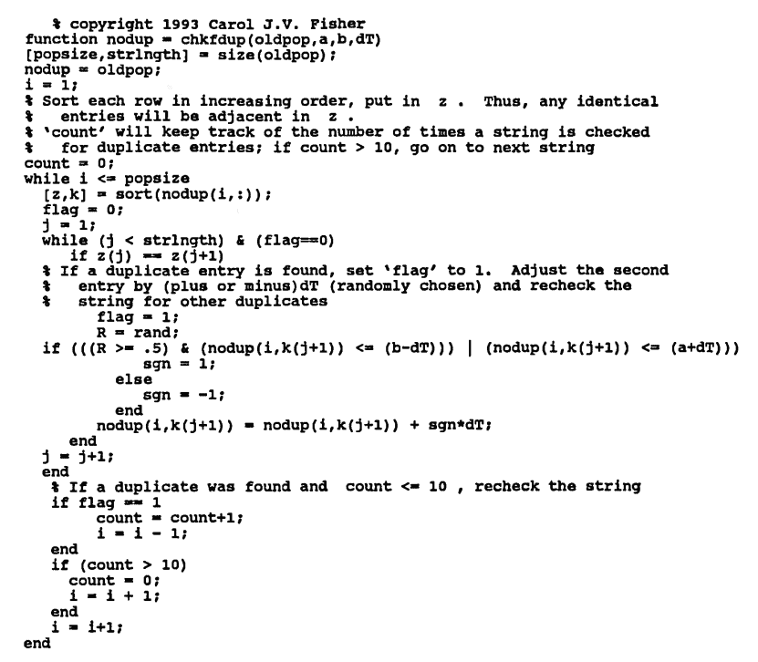
$(5)$ The periods in each string $\,(P_1,\ldots,P_m)\,$ must be distinct. Otherwise, when linear least-squares techniques are applied, the matrix $\,X\,$ will have duplicate columns, and hence be singular (Section 2.2).
The MATLAB function chkfdup checks each string for duplicate periods. Entries are (randomly) adjusted by $\,\pm\Delta T\,$ to correct any duplicate values. The code for the function chkfdup is included at the end of this section.
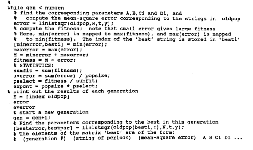
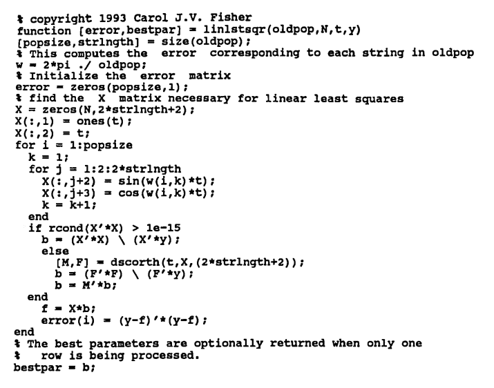
$(6)$ The function linlstsqr finds the parameters $\,A\,,$ $\,B\,,$ $\,C_i\,$ and $\,D_i\,$ $\,(i = 1,\ldots,m)\,$ corresponding to each string $\,(P_1,\ldots,P_m)\,$ in oldpop , and computes the associated mean-square error. These errors are returned in the matrix error . The code for the function linlstsqr is included at the end of this section.
$(7)$ The average error (averror) for the initial population is computed by summing the individual errors, and dividing by the number of strings.
$(8)$ The least error, over all the strings, is returned as minerror . The row number of the corresponding least-error string is returned in besti . If more than one row has the same least error, then the first such row is returned.
$(9)$ The greatest error, over all the strings, is returned as maxerror .
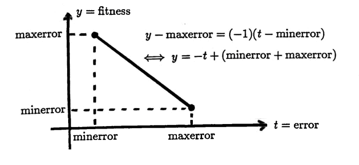
$(10$–$11)$ The fitness of each string is computed via the linear function below. Observe that minimum error is mapped to maximum fitness, and maximum error is mapped to minimum fitness.
$(12)$ The ‘population fitness’ sumfit is the sum of the fitnesses of each string in the population.
$(13)$ The probability that a given string will be selected for the next generation is given by its fitness, divided by the population fitness.
$(14)$ The (theoretical) expected number of each string in the subsequent population is found by multiplying the probability of selection by the population size.
Example
Let D be the data set formed by these commands:
t = [0:.1:20]';
y = 1 + .5*t + sin(2*pi*t/5)
- 2*cos(2*pi*t/5)
+ 7*cos(2*pi*t/17);
noise = 2*(rand(t) - .5);
y = y + noise;
D = [t y];
The reader will recognize this data set from the previous MATLAB example of the gradient method. The sinusoids have periods $\,5\,$ and $\,17\,.$
Let a $= 1\,,$ b $= 20\,,$ dT $= 0.5\,,$ popsize $= 10\,,$ strlngth $= 2\,,$ and numgen $= 3\,.$ An application of
best = genetic(D,a,b,dT,popsize,strlngth,numgen)
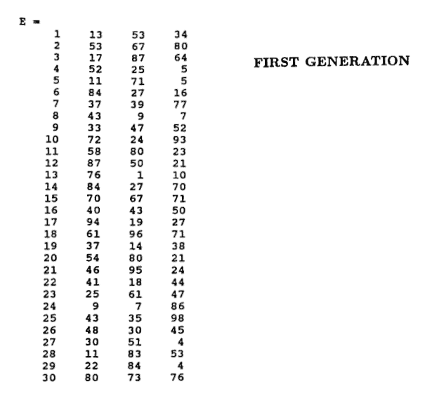
(modified to print out more information than usual), yielded the following initial population, associated mean-square errors, fitness, probability of selection, and expected count in the next population:
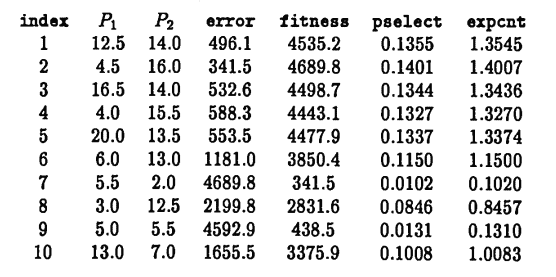
Observe that the numbers $\,P_1\,$ and $\,P_2\,$ are randomly distributed between $\,1\,$ and $\,20\,,$ with increment $\,0.5\,.$ The string with the least error is $\,[4.5 \ \ 16.0]\,$; not surprisingly, since these periods are close to the actual periods $\,5\,$ and $\,17\,.$
The average error for this initial population is:
$$ \begin{align} &\boldsymbol{\rm averror}\cr\cr &\quad = \frac{496.1+ 341.5 + \cdots + 1655.5}{10}\cr\cr &\quad = 1683.1 \end{align} $$Observe that small error corresponds to high fitness, and strings with high fitness have a greater probability of selection (pselect) and expected count (expcnt) in the next generation. The sum of the fitnesses for this first generation is:
$$ \begin{align} &\boldsymbol{\rm sumfit}\cr &\quad = 4535.2 + 4689.8 + \cdots + 3375.9\cr &\quad = 33482.6 \end{align} $$Notice that most of the ‘high-fitness’ strings seem to have a period close to $\,17\,.$ This is because the amplitude of the period-$17$ sinusoid in the ‘known unknown’ is $\,7\,,$ whereas the amplitude of the period-$5$ sinusoid is only $\,\sqrt{1^2 + (-2)^2} = \sqrt 5\,.$ In general, periods corresponding to larger amplitude sinusoids will have a greater influence on the string fitness.
As written, the function genetic does not scroll all the information given in the previous example. It scrolls only the information:
E = [index oldpop]
error
averror
while it is running. This information can be captured by typing diary before running genetic .
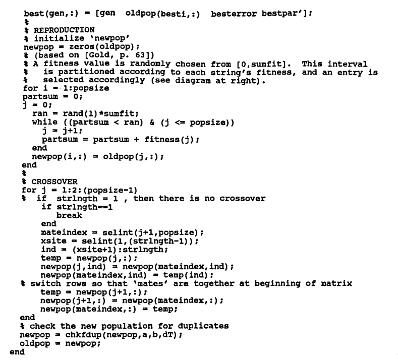
After producing the initial population and statistics, reproduction takes place.
(REPRODUCTION) The initial population is reproduced, based on the fitness of its strings.
The following reproduction scheme is adapted from [Gold, p. 63].
The interval $\,[0,\boldsymbol{\rm sumfit}]\,$ is partitioned, according to the fitness of each string. Let $\,\boldsymbol{\rm fit}(i)\,$ denote the fitness of string $\,i\,,$ for $\,i = 1,\ldots,\boldsymbol{\rm popsize}\,.$ The sketch below shows the partitioning of $\,[0,\boldsymbol{\rm sumfit}] = [0,33482.6]\,$ corresponding to the initial population in the previous example:
![partitioning of the interval [0,sumfit]](graphics/S2_4Img19.png)
With this partition in hand, a number is selected randomly (using a uniform distribution) from the interval $\,[0,\boldsymbol{\rm sumfit}]\,.$ If the number lands in the subinterval corresponding to string $\,i\,,$ then a copy of string $\,i\,$ is placed in the next population. This process is repeated popsize times to complete reproduction.
The following MATLAB code implements the ideas just discussed:
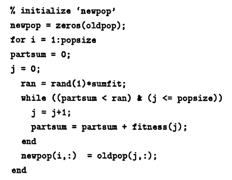
Octave requires:
newpop = zeros(size(oldpop));
To eliminate Octave's short-circuit warnings, use the scalar logical operator && instead of & .
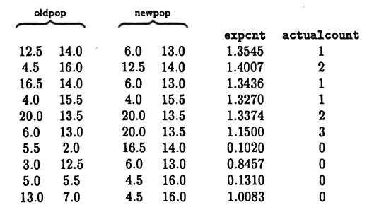
Example (continued)
Shown below is the initial population, oldpop , and the reproduced population, newpop . Also shown is the expected count, expcnt , of each string in oldpop , and the actual count, as observed from newpop :
(CROSSOVER) The final step in this simple genetic algorithm is crossover, where the strings in newpop are ‘matched up and mixed’ to try and achieve an optimal string, as follows:
The first string in newpop is ‘mated’, at random, with another (different index) string from newpop . Then, a ‘crossover site’ is chosen at random from the set $\,\{1,2,\ldots,(\boldsymbol{\rm strlngth}- 1)\}\,.$ The information to the right of this ‘crossover site’ is swapped, as illustrated next:
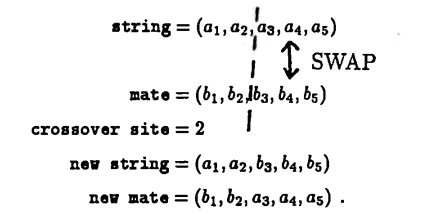
Once mated and swapped, the first string's (adjusted) mate is placed in row $(2)$ of the new population. The procedure is then repeated with the remaining strings.
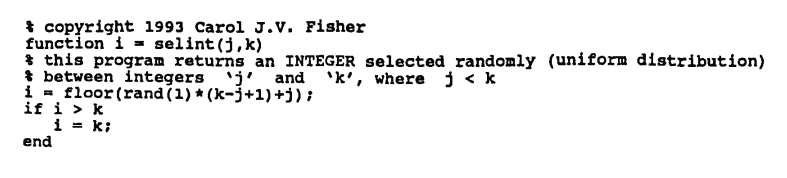
In order to implement crossover, it is necessary to have a way to randomly select an integer between prescribed bounds. The following MATLAB function accomplishes this:
MATLAB
FUNCTION
selint
Let
j
and
k
be integers, with
j $\lt$
k .
The command
i = selint(j,k)
returns an integer
i
selected randomly from the interval
[j,k].
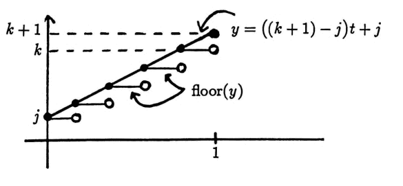
function i = selint(j,k)
i = floor(rand(1)*(k-j+1)+j);
if i $\gt$ k
i = k;
end
For Octave, you must add endfunction as the last line.
Recall that rand(1) returns a number selected randomly from $\,[0,1]\,,$ using a uniform distribution. Also recall that floor(x) returns the greatest integer less them or equal to x .
The graph below illustrates how the integer between j and k is selected:
Example (continued)
Shown below is newpop before crossover, and after crossover. The arrows indicate the strings that were mated. Observe that when strlngth $\,= 2\,,$ the crossover site is always $\,1\,.$
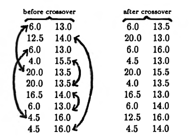
Since it is possible to have duplicate values after crossover, newpop is checked for duplicates before continuing with the algorithm.
The average error in this reproduced, crossed-over population is $\,792.2\,,$ as compared to $\,1683.1\,$ for the old population. Thus, the ‘fitness’ of the overall population has indeed improved!
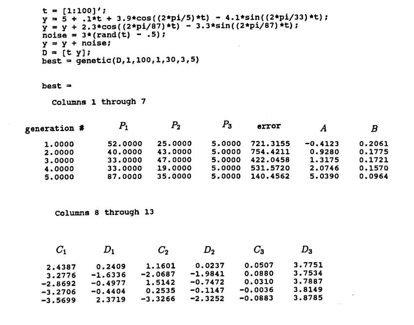
Diary of an Actual MATLAB Session
The following diary of an actual MATLAB session begins by constructing a ‘known unknown’ consisting of sinusoids with periods $\,5\,,$ $\,33\,$ and $\,87\,,$ and with close amplitudes. The search for periods is done on the interval $\,[1,100]\,$ with increment $\,1\,.$ A population size of $\,30\,$ is used. Five generations are computed.
By the fifth generation, components with periods $\,5\,,$ $\,35\,$ and $\,87\,$ were ‘found’ with an associated error of only $\,\approx 140\,.$ What is the probability that this good a result would have been obtained by random choice alone?
The parameter space has $\,(100)^3\,$ elements, since there are $\,100\,$ choices for periods in the interval $\,[1,100]\,$ with interval $\,1\,.$ Each generation uses $\,30\,$ points in this space, so $\,5\,$ generations yield $\,5\cdot 30 = 150\,$ points in parameter space.
Consider a ‘box’ around the actual solution point $\,(5,33,87)\,,$ where each coordinate lies within $\,2\,$ of the actual solution point:
$$ \{3,4,5,6,7\} \times \{31,32,33,34,35\} \times \{85,86,87,88,89\} $$There are $\,5^3 = 125\,$ such points. By merely randomly choosing points in space, the probability of hitting a point in this ‘box’ on a single draw is $\,\frac{125}{(100)^3} = 0.000125\,.$
On $\,N\,$ draws, what is the probability of hitting a point within this box?
$$ \begin{align} &P[(\text{point in box on draw #1})\cr &\qquad \text{OR}\ (\text{point in box on draw #2})\cr &\qquad \text{OR}\ \cdots\cr &\qquad \text{OR}\ (\text{point in box on draw #$N$})]\cr\cr &\quad = 1 - P(\text{point is NOT in box on all $\,N\,$ draws})\cr\cr &\quad = 1 - (1 - 0.000125)^N\cr\cr &\quad \approx 0.0186\,, \text{when}\ N = 150 \end{align} $$Thus, the probability of hitting a point in the box on $\,150\,$ draws, by random search alone, is less than $\,2\%\,$! This example illustrates the power of the genetic algorithm.
It is again noted that if one sinusoid has an amplitude considerably larger than others in the sum, then that sinusoid gets ‘favored’ in the search process.
The summary of the ‘best’ choices from each generation, together with the first generation, are shown.
noise = 3*(rand(size(t)) - .5);
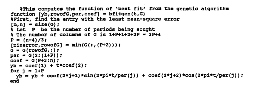
The function bfitgen (‘best fit from the genetic algorithm’) is convenient for plotting the best approximation obtained from an application of the genetic algorithm:
G = genetic(D,a,b,dT,popsize,strlgnth,numgen);
To use the function bfitgen, type:
[yb,rowofG,per,coef] = bfitgen(t,G);
The required inputs are:
- the matrix G from an application of the genetic algorithm;
- a column vector t used to compute the data values of the best approximation. Often, one uses: t = D(:,1)
-
The column vector yb contains the values of the best approximation. To plot this best approximation, type either:
plot(t,yb) or plot(t,yb,'x')
- The optional outputs rowofG , per , and coef contain, respectively: the generation number in which the best approximation was obtained; the periods P1 $\cdots$ Pm of the best approximation; the corresponding coefficients A B C1 D1 $\cdots$ Cm Dm of the best approximation.
The Programs
The code for genetic and the necessary auxiliary functions is given next:
Octave requires two line changes:
% REQUIRED in Octave
newpop = zeros(size(oldpop));
% To eliminate Octave's warnings:
while ((partsum < ran) && (j <= popsize))
% && is for scalar logic, which is what we're using
Octave also requires endfunction as the last line of genetic .
Octave requires:
X(:,1) = ones(size(t));
Octave also requires endfunction as the last line of linlstsqr .
To eliminate Octave's short-circuit warnings, use the scalar logical operators && and || .
Octave requires endfunction as the last line of chkfdup .
Note that this chkfdup function is different than the function suggested in Section 1.2 .