2.2 Tests for Specific Conjectured Components: Linear Least-Squares Approximation
In certain instances, a researcher may conjecture that a data set $\,\{(t_i,y_i)\}_{i=1}^N\,$ will be well-modeled by a function of a specified form. This conjecture may arise from a combination of experience, initial data inspection, or knowledge of the mechanisms generating the data.
For example, the data set graphed below shows a linear trend, and one might reasonably seek constants $\,m\,$ and $\,b\,$ so that the function $\,f(x) = mx + b\,$ ‘fits’ the data well. (The notion of ‘fit’ is addressed precisely in this section.)
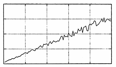
LINEAR TREND
As a second example, the data set graphed below appears to have a global quadratic component. There also seems to be some interesting local periodic behavior—the curve seems to oscillate about a parabola. These observations might lead one to suspect that there are constants $\,a\,,$ $\,b\,$ and $\,c\,$ for which the function
$$ \begin{align} y(t) &= \overbrace{at^2 + bt + c}^{\text{quadratic component}}\cr &\qquad + \lt\text{some periodic component}\gt \end{align} $$will give a good ‘fit’ to the data. A researcher might attempt to identify the quadratic component, and then subtract it off, in order to isolate and study the more local periodic behavior.
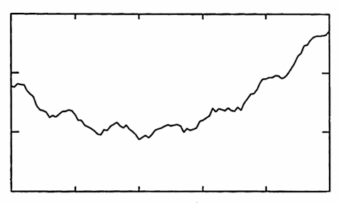
QUADRATIC TREND
(Fitting function passes through each data point)
There are many ways to quantify the notion of ‘fitting’ a data set $\,\{(t_i,y_i)\}_{i=1}^N\,$ with a function $\,f\,.$ One very strong condition is to require that the function $\,f\,$ pass through every data point; i.e., $\,f(t_i) = y_i\,$ for all $\,i\,.$ The process of finding such a function is called interpolation; and the resulting function is called an interpolate (of the data set).
As illustrated below, there are many possible interpolates for a given data set. Usually, the interpolating function is selected to have some additional desirable properties.
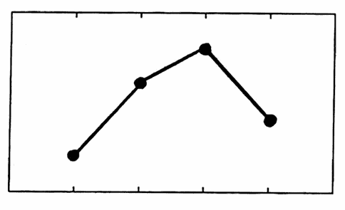
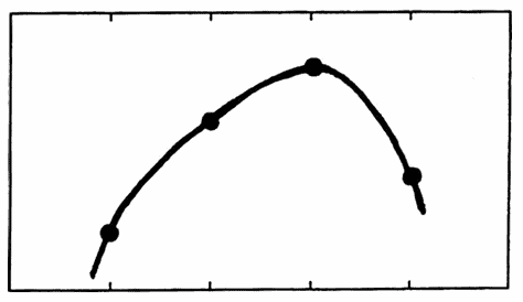
TWO INTERPOLATES OF A DATA SET
For example, the interpolate may be required to be a single polynomial (see Section 2.5). Polynomial interpolation has the disadvantage that one often gets large oscillations between the data points.
To avoid such oscillations, one can alternatively use cubic polynomials that are appropriately ‘patched together’ at the data points—the resulting interpolate is called a cubic spline, and is also discussed in Section 2.5. Interpolates are often used to supply missing data values.
The exact matching required in interpolation may not be possible if a function of a specific form is desired; for example, no linear function $\,f(x) = mx+b\,$ can be made to pass through three non-collinear points.
More importantly, such exact matching may not even be justified in situations where each data value is potentially ‘contaminated’ by noise. In such cases, it often makes more sense to seek a function that merely ‘comes close’ to the data points—this leads to a method of ‘fitting’ a data set that is commonly called approximation.
‘Objects being close’ is made precise via a norm
One way to make precise the notion of ‘objects being close’ in mathematics is by the use of a norm. Roughly, a norm is a function that measures the size of an object; the ‘size’ of $\,x\,$ is often denoted by $\,\|x\|\,$ and read as ‘the norm of $\,x\,$’.
The norm (and underlying vector space structure) then allows one to talk about the distance between objects; the distance between $\,x\,$ and $\,y\,$ is $\,\|x-y\|\,.$ The objects $\,x\,$ and $\,y\,$ are ‘close’ (with respect to the given norm) if $\,\|x-y\|\,$ is small.
Appendix 2 gives the precise definitions of a norm, a vector space, and related results.
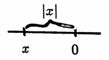
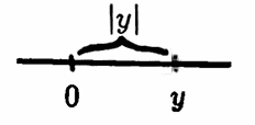
For example, the absolute value function is a norm on the real numbers. For every real number $\,x\,,$ the nonnegative number $\,|x|\,$ ‘measures’ $\,x\,$ by giving its distance from zero on the real number line.
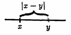
Given any real numbers $\,x\,$ and $\,y\,,$ the distance between them is $\,|x - y|\,$; so $\,x\,$ and $\,y\,$ are ‘close’ (with respect to the absolute value norm) if $\,|x - y|\,$ is small.
Let $\,\Bbb R^n\,$ denote all $n$-tuples of real numbers:
$$ \Bbb R^n := \{(x_1,\ldots,x_n)\ |\ x_i\in\Bbb R\,,\ 1\le i\le n\} $$Addition and subtraction of $n$-tuples is done componentwise. Elements of $\,\Bbb R^n\,$ are commonly called vectors (since $\,\Bbb R^n\,$ is a vector space).
Let $\,\boldsymbol{\rm x}\,$ denote a typical element in $\,\Bbb R^n\,.$ A norm on $\,\Bbb R^n\,$ is given by:
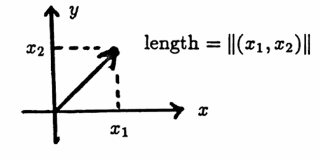
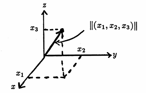
$$ \|\boldsymbol{\rm x}\| := \sqrt{x_1^2 + \cdots + x_n^2} \tag{1} $$This norm is called the Euclidean norm; the Euclidean norm of an $n$-tuple is the square root of the sum of its squared entries.
When $\,n\,$ equals $\,2\,$ or $\,3\,,$ the nonnegative number $\,\|\boldsymbol{\rm x}\|\,$ has a nice geometric interpretation—it gives the length of the arrow from the origin to the point with coordinates $\,\boldsymbol{\rm x}\,.$
Two $n$-tuples $\,\boldsymbol{\rm x}\,$ and $\,\boldsymbol{\rm y}\,$ are ‘close’ (with respect to the given norm) if $\,\|\boldsymbol{\rm x} - \boldsymbol{\rm y}\|\,$ is small.
In this dissertation, whenever an element of $\,\Bbb R^n\,$ is used in the context of matrix manipulations, it will be represented as a column vector.
Letting $\,\boldsymbol{\rm y}\,$ be the column vector
$$ \boldsymbol{\rm y} := \begin{bmatrix} y_1 \\ y_2 \\ \vdots \\ y_n \end{bmatrix}\ , $$then $\,\boldsymbol{\rm y}^t\,$ ($\,\boldsymbol{\rm y}\,$ transpose) is the row vector
$$ \begin{bmatrix} y_1 & y_2 & \cdots & y_n \end{bmatrix}\ , $$and the Euclidean norm of $\,\boldsymbol{\rm y}\,,$ squared, is displayed in matrix notation as:
$$ \begin{align} \|\boldsymbol{\rm y}\|^2 &= y_1^2 + \cdots + y_n^2\cr &= [y_1\ y_2\ \cdots\ y_n] \begin{bmatrix} y_1 \\ y_2 \\ \vdots \\ y_n \end{bmatrix} \cr &= \boldsymbol{\rm y}^t\boldsymbol{\rm y} \end{align} $$A function $\,f\,$ is said to approximate a data set $\,\{(t_i,y_i)\}_{i=1}^N\,$ if it is ‘close to’ the data set, in some normed sense. The process of finding such a function is called approximation. The sketches below illustrate two types of approximation.
Least-squares approximation, discussed in this and the next two sections, is so-called because it seeks a function that minimizes the sum of the squared distances between the approximating function and the data set.
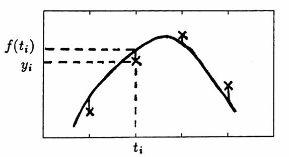
$$ \underset{f}{\text{minimize}} \left( \sum_i \bigl( y_i - f(t_i) \bigr)^2 \right) $$
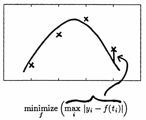
Minimax (or Chebyshev) approximation seeks to minimize the maximum distance between the data set and approximating function; although simply stated, the mathematics is difficult, and minimax approximation is not discussed here.
The method of least squares arises when the Euclidean norm $\,(1)\,$ is used for approximation, as follows.
Let $\,\cal F\,$ be a set of real-valued functions of one real variable, the members of which are to serve as candidates for approximation of the data set $\,\{(t_i,y_i)\}_{i=1}^N\,.$
Denote a typical function in $\,\cal F\,$ by $\,f\,,$ and let $\,\boldsymbol{\rm f}\,$ denote the $N$-tuple $\,\bigl(f(t_1),\ldots,f(t_N)\bigr)\,,$ formed by letting $\,f\,$ act on the $\,N\,$ time values $\,(t_1,\ldots,t_N)\,.$
The $N$-tuple of data values $\,\boldsymbol{\rm y} := (y_1,\ldots,y_N)\,$ can be compared to the $N$-tuple $\,\boldsymbol{\rm f}\,$ via the Euclidean norm given in $\,(1)\,$:
$$ \begin{align} &\|\boldsymbol{\rm y} - \boldsymbol{\rm f}\|\cr\cr &\quad = \|(y_1,\ldots,y_N) - \bigl(f(t_1),\ldots,f(t_N)\bigr)\|\cr\cr &\quad = \|\bigl( y_1-f(t_1),\ldots,y_N - f(t_N) \bigr)\|\cr\cr &\quad = \sqrt{ \sum_{i=1}^N \bigl( y_i - f(t_i) \bigr)^2} \end{align} \tag{2} $$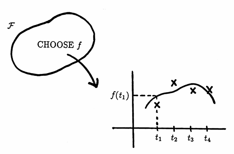
The sum in $\,(2)\,$ is nicely interpreted as the error between the function $\,f\,$ and the data set . Allowing $\,f\,$ to vary over all the members in $\,\cal F\,,$ one can investigate the corresponding errors.
If a function $\,\hat f\,$ can be found that minimizes this error, then it is called a least-squares approximate, from $\,f\,,$ to the data set. For such a function $\,\hat f\,,$ with corresponding $N$-tuple $\,\hat{\boldsymbol{\rm f}} := \bigl( \hat f(t_1),\ldots,\hat f(t_N) \bigr)\,,$
$$ \|\boldsymbol{\rm y} - \hat{\boldsymbol{\rm f}}\| = \underset{f\in\cal F}{\text{min}} \|\boldsymbol{\rm y} - \boldsymbol{\rm f}\|\,, $$so that, for all $\,f\in \cal F\,$:
$$ \|\boldsymbol{\rm y} - \hat{\boldsymbol{\rm f}}\| \le \|\boldsymbol{\rm y} - \boldsymbol{\rm f}\| $$Since $\,\hat f\,$ minimizes the error, it is a best approximation to the data set from $\,\cal F\,.$ If $\,\hat f\,$ is unique, then it is the best approximation from $\,\cal F\,.$
If the set $\,\cal F\,$ contains a finite number of functions, then such a minimizing function $\,\hat f\,$ can always be found (but may not be unique). In most interesting applications of least-squares approximation, however, the set $\,\cal F\,$ contains an infinite number of functions, and existence and uniqueness of a best approximation is more delicate.
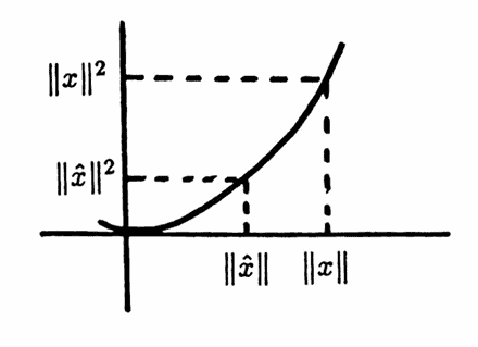
The appearance of the square root in $\,(2)\,$ is bothersome, and can be avoided by a simple observation, which is:
Let $\,X\,$ be any set on which a norm is defined. If there exists $\,\hat x\in X\,$ for which
$$ \|\hat x\| = \underset{x\in X}{\text{min}} \|x\|\,, $$then:
$$ \|\hat x\|^2 = \underset{x\in X}{\text{min}} \|x\|^2 $$Conversely, if $\|\hat x\|^2 = {\text{min}}_{x\in X} \|x\|^2\,,$ then $\|\hat x\| = {\text{min}}_{x\in X} \|x\|\,.$
Proof
Suppose there exists $\,\hat x\in X\,$ for which $\,\|\hat x\| = {\text{min}}_{x\in X} \|x\|\,.$ Then:
$$ \|\hat x\| \le \|x\|\ \ \text{for all}\ x\in X $$Since the squaring function $\,f(x) = x^2\,$ increases on $\,[0,\infty)\,,$ it follows that
$$ \|\hat x\|^2 \le \|x\|^2\ \ \text{for all}\ x\in X\,, $$from which $\,\|\hat x\|^2 = {\text{min}}_{x\in X} \|x\|^2\,.$
The converse uses the fact that the square root function increases on $\,[0,\infty)\,.$ $\blacksquare$
With this observation, the approximation problem
$$ \underset{f\in\cal F}{\text{min}}\, \|\boldsymbol{\rm y} - \boldsymbol{\rm f}\| $$can always be replaced by the equivalent problem
$$ \underset{f\in\cal F}{\text{min}}\, \|\boldsymbol{\rm y} - \boldsymbol{\rm f}\|^2\ , $$whenever it is convenient to do so. Such a replacement eliminates the bothersome square root sign in $(2)\,.$
A frequently-occurring case of least-squares approximation is discussed next, together with its MATLAB implementation.
Suppose that a data set $\,\{(t_i,y_i)\}_{i=1}^N\,$ and $\,m\,$ real-valued functions of one real variable, $\,f_1,\ldots,f_m\,,$ are given. Let
$$ {\cal F} := \{c_1f_1 + \cdots + c_mf_m\ |\ c_i\in\Bbb R\,,\, 1\le i\le m\} $$be the class of functions to be used in approximating the data set. Note that each function in $\,\cal F\,$ is a linear combination of the functions $\,f_1,\ldots,f_m\,$; hence the name linear least-squares approximation.
However, the functions $\,f_i\,$ certainly need not be linear functions; in many practical applications, the $\,f_i\,$ will be polynomials or sinusoids. The function $\,f_1\,$ is usually taken to be $\,f_1(t) \equiv 1\,,$ to allow for a constant term in the approximating function.
The goal of least-squares approximation is to find real constants $\,b_1,\ldots,b_m\,$ so that the function $\,f\,$ given by
$$ f(t) := b_1f_1(t) + b_2f_2(t) + \cdots + b_mf_m(t) $$minimizes the sum:
$$ \sum_{i=1}^N \bigl( y_i - f(t_i)\bigr)^2 $$Evaluation of the function $\,f\,$ at the $\,N\,$ time values $\,t_1,\ldots,t_N\,$ yields $\,N\,$ equations:
$$ \begin{align} f(t_1) &= b_1f_1(t_1) + b_2f_2(t_1) + \cdots + b_mf_m(t_1)\cr f(t_2) &= b_1f_1(t_2) + b_2f_2(t_2) + \cdots + b_mf_m(t_2)\cr &\ \, \, \vdots\cr f(t_N) &= b_1f_1(t_N) + b_2f_2(t_N) + \cdots + b_mf_m(t_N) \end{align} \tag{3} $$By defining
$$ \begin{gather} \boldsymbol{\rm f} := \begin{bmatrix} f(t_1) \\ \vdots \\ f(t_N) \end{bmatrix}\ ,\cr \cr \boldsymbol{\rm X} := \begin{bmatrix} f_1(t_1) & \cdots & f_m(t_1) \\ f_1(t_2) & \cdots & f_m(t_2) \\ \vdots & \vdots & \vdots \\ f_1(t_N) & \cdots & f_m(t_N) \end{bmatrix}\ ,\cr \cr \text{and}\cr \cr \boldsymbol{\rm b} := \begin{bmatrix} b_1 \\ \vdots \\ b_m \end{bmatrix}\ , \end{gather} $$the system in $\,(3)\,$ can be written as:
$$ \boldsymbol{\rm f} = \boldsymbol{\rm X}\boldsymbol{\rm b} $$The sizes of the matrices $\,\boldsymbol{\rm f}\,,$ $\,\boldsymbol{\rm X}\,,$ and $\,\boldsymbol{\rm b}\,$ are, respectively, $\,N \times 1\,,$ $\,N\times m\,,$ and $\,m\times 1\,.$
Define $\,\boldsymbol{\rm y}\,$ to be the column vector of data values:
$$ \boldsymbol{\rm y} := \begin{bmatrix} y_1 \\ \vdots \\ y_N \end{bmatrix} $$Then, $\,\boldsymbol{\rm y}\,$ has size $\,N \times 1\,,$ as does $\,\boldsymbol{\rm y} - \boldsymbol{\rm X}\boldsymbol{\rm b}\,.$
The least-squares problem is to minimize
$$ \begin{align} \text{SSE} &:= \|\boldsymbol{\rm y} - \boldsymbol{\rm f}\|^2\cr &= \|\boldsymbol{\rm y} - \boldsymbol{\rm X}\boldsymbol{\rm b}\|^2\cr &= (\boldsymbol{\rm y} - \boldsymbol{\rm X}\boldsymbol{\rm b})^t (\boldsymbol{\rm y} - \boldsymbol{\rm X}\boldsymbol{\rm b})\ , \end{align} $$where SSE stands for ‘sum of the squared errors’. SSE is to be viewed as a function from $\,\Bbb R^m\,$ into $\,\Bbb R\,$; it takes an $m$-tuple $\,\boldsymbol{\rm b}\,$ and maps it to the real number $\,(\boldsymbol{\rm y} - \boldsymbol{\rm X}\boldsymbol{\rm b})^t (\boldsymbol{\rm y} - \boldsymbol{\rm X}\boldsymbol{\rm b})\,.$
Indeed, SSE is a differentiable function of $\,\boldsymbol{\rm b}\,$ [G&VL, 221ff]. Therefore, a necessary condition to minimize SSE is that its partial derivatives with respect to the components $\,b_i\,$ of $\,\boldsymbol{\rm b}\,$ equal zero.
Appendix 3 shows that the partial derivatives of SSE are contained in the $m$-column vector:
$$ 2(\boldsymbol{\rm X}^t\boldsymbol{\rm X}\boldsymbol{\rm b} - \boldsymbol{\rm X}^t\boldsymbol{\rm y}) $$Therefore, a minimizing vector $\,\boldsymbol{\rm b}\,$ must satisfy
$$ \boldsymbol{\rm 0} = 2(\boldsymbol{\rm X}^t\boldsymbol{\rm X}\boldsymbol{\rm b} - \boldsymbol{\rm X}^t\boldsymbol{\rm y}) \ , $$or, equivalently:
$$ \boldsymbol{\rm X}^t\boldsymbol{\rm X}\boldsymbol{\rm b} = \boldsymbol{\rm X}^t\boldsymbol{\rm y} $$If $\,\boldsymbol{\rm X}^t\boldsymbol{\rm X}\,$ is invertible, then
$$ \boldsymbol{\rm b} = (\boldsymbol{\rm X}^t\boldsymbol{\rm X})^{-1}\boldsymbol{\rm X}^t\boldsymbol{\rm y} $$gives the unique least-squares parameters. Observe that the matrix $\,\boldsymbol{\rm X}^t\boldsymbol{\rm X}\,$ is an $\,m \times m\,$ real symmetric matrix; the invertibility of $\,\boldsymbol{\rm X}^t\boldsymbol{\rm X}\,$ is discussed in Section 2.3 and Appendix 2.
A MATLAB procedure for finding the least-squares parameters $\,\boldsymbol{\rm b}\,$ is discussed next.
MATLAB IMPLEMENTATION: Linear Least-Squares Approximation
Purpose and Notation
Let $\,\{(t_i,y_i)\}_{i=1}^N\,$ be a given data set, and let $\,f_1,\ldots,f_m\,$ be $\,m\,$ real-valued functions of a real variable.
Define:
$$ \begin{align} \boldsymbol{\rm t} &:= (t_1,\ldots,t_N)\,,\cr\cr \boldsymbol{\rm y} &:= (y_1,\ldots,y_N)\,,\cr\cr f(t) &:= b_1f_1(t) + \cdots + b_mf_m(t)\cr &\qquad \text{for}\ b_i\in\Bbb R\,,\ 1\le i\le m\,,\ \text{and}\cr\cr \boldsymbol{\rm f} &:= \bigl( f(t_1),\ldots,f(t_N) \bigr) \end{align} $$The linear least-squares approximation problem is to find specific choices for $\,b_1,\ldots,b_m\,$ so that the error
$$ \|\boldsymbol{\rm y} - \boldsymbol{\rm f}\|^2 = \sum_{i=1}^N \bigl( y_i - f(t_i)\bigr)^2 $$is minimized.
Required Inputs
- The $\,N\,$ time values $\,t_i\,$ are stored in an $N$-column vector called t .
- The $\,N\,$ data values $\,y_i\,$ are stored in an $N$-column vector called y .
MATLAB Commands
The following list of MATLAB commands will produce (under suitable conditions) a column vector b with entries $\,b_1,\ldots,b_m\,$ so that $\,f(t) = b_1f_1(t) + \cdots + b_mf_m(t)\,$ gives the least-squares approximate to the data set.
The actual data set is plotted on the same graph with the best approximating function, and the least-squares error is computed.
The example following these commands explains and illustrates the procedure.

Example
The following list of MATLAB commands produces a set of ‘noisy’ data of the form
$$ y(t) = 3.2 - 0.7t + 0.05t^2 + \sin\frac{2\pi t}{3} + \langle\text{noise}\rangle $$which is the ‘known unknown’. A least-squares approximate of the form
$$ f(t) = b_1 + b_2t + b_3t^2 + b_4t^3 + b_5t^4 $$is computed. There are $\,5\,$ approximating component functions:
$$ \begin{gather} f_1(t) = 1\cr f_2(t) = t\cr f_3(t) = t^2\cr f_4(t) = t^3\cr f_5(t) = t^4 \end{gather} $$The actual data set is graphed together with its least-squares approximate, and the error is computed.
Based on an analysis of the difference between the actual data and the approximate, the form of the approximating function is updated, and a second least-squares approximate is obtained, which gives a beautiful fit to the actual data.
The lines are numbered for easy reference in the discussion that follows.
Octave requires minor changes on two lines:
2) N = .5*(2*rand(size(t)) - 1);
5) f1 = ones(size(t));
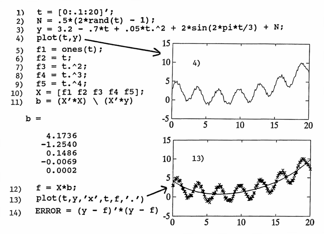
1) A time vector is created; entries begin at $\,0\,,$ are evenly spaced with spacing $\,0.1\,,$ and end at $\,20\,.$ The prime mark $\,'\,$ denotes the transpose operation, and makes t a column vector. The semicolon (;) at the end of the line suppresses MATLAB echoing.
2) N (for ‘Noise’) is a column vector the same size as t with entries uniformly distributed on $\,[-0.5, 0.5]\,.$
3) The data values y are computed. Recall that t.^2 gives a MATLAB array operation; each element in t is squared.
4) The data set is plotted as a line graph. That is, MATLAB ‘connects the points’ with a curve.
5) The first function is $\,f_1(t) \equiv 1\,.$ The MATLAB command ones(t) produces a vector the same size as t , with all entries equal to $\,1\,.$
6-9) The functions $\,f_2(t) = t\,,$ $\,f_3(t) = t^2\,,$ $\,f_4(t) = t^3\,$ and $\,f_5(t) = t^4\,$ are evaluated at the appropriate time values.
10) The matrix X is formed by laying the column vectors f1 through f5 next to each other.
11) The least-squares parameters b are computed. The backslash operator $\,\backslash\,$ provides a way of doing ‘matrix division’ that is more efficient than calculating the inverse of a matrix.
More precisely, solving Ax = b via the MATLAB command
x = inv(A) * b
would cause MATLAB to calculate the inverse of A , and then multiply by b .
However, solving Ax = b via the MATLAB command
x = A \ b
(to understand this, read it from right to left as ‘ b divided by a ’) solves the system using Gaussian elimination, without ever calculating the inverse of A . This method is greatly preferred from a numerical accuracy and efficiency standpoint.
Since there is no semicolon at the end of the line to suppress MATLAB echoing, the column vector b is printed.
12) The least-squares approximate is computed at the time values of the data set, and called f .
13) The actual data is point-plotted with the symbol ‘ x ’; on the same graph, the least-squares approximate is point-plotted with the symbol ‘ . ’ .
14) The least-squares error is computed and printed.
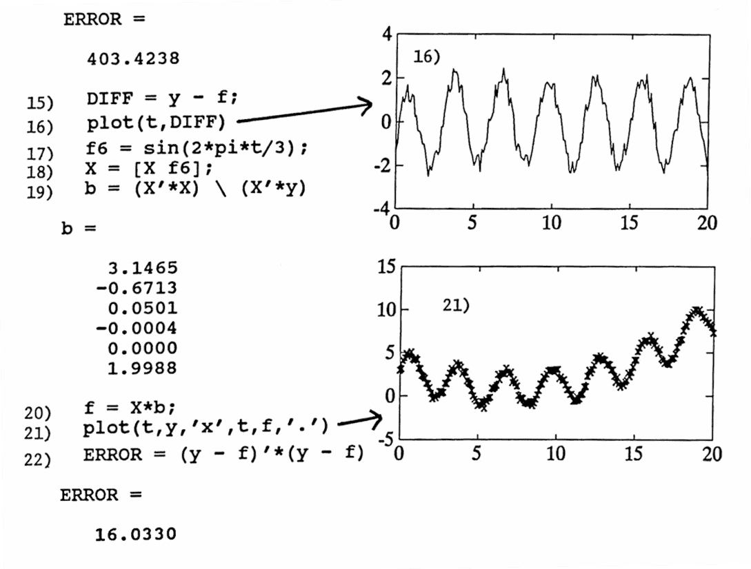
15–16) The difference between the actual data and approximating function is computed as DIFF , and plotted.
17–18) Visual inspection shows that the difference seems to be a sinusoid of period $\,3\,.$ (Alternatively, techniques discussed later on in this dissertation can be used to reach this conclusion; see Section $2.6$). Thus, least-squares is applied again with an additional function $\,f_6(t) = \sin\frac{2\pi t}3\,.$ The new column vector f6 is computed, and X is updated by concatenating this new column vector.
19–21) The new least-squares parameters and function are computed, and a graph showing the ‘fit’ is plotted.
22) The new ERROR is computed, confirming that a beautiful fit has been achieved.
If desired, the procedure described here can be automated into a MATLAB m-file.
As the number of component functions $\,f_1,f_2,\ldots,f_m\,$ increases, the matrix $\,X^tX\,$ often approaches singularity; that is, it looks more and more like a noninvertible matrix. This can cause the procedure just described to break down. In the next section, the matrix $\,X^tX\,$ is studied in more detail, and the concept of orthogonal functions is introduced as a method of overcoming the ‘near singularity’ of $\,X^tX\,.$