1.2 Notation
In this section, notation is developed that will be used throughout the dissertation.
Many data sets consist of a collection of ordered pairs of real numbers: each ordered pair $\,(t,y)\,$ in the collection contains an input to some data-generation process, denoted by $\,t\,,$ and its corresponding output from the data-generation process, denoted by $\,y\,.$
In this dissertation, the word ‘time’ is used to refer to inputs.
The data sets to be studied in this dissertation have the additional property that the times can be listed; and, they can be listed in increasing order. This leads to the definition of discrete-domain data, stated next:
A set of ordered pairs with real-number entries is called a discrete-domain data set, if the following conditions hold:
- The total number of ordered pairs in the set is either finite, or countably infinite (i.e., can be put in a one-to-one correspondence with the positive integers). Thus, the set can be notated as $\,\{(t_i,y_i)\}_{i=1}^N\,$ if it is finite; or $\,\{(t_i,y_i)\}_{i=1}^\infty\,,$ if it is countably infinite.
- The time values, $\,\{t_i\}_{i=1}^{(N\text{ or }\infty)}\,$ can be arranged in strictly increasing order. In particular, the time values are all distinct.
MATLAB commands for checking that the time values in a finite data set are distinct, and re-ordering the ordered pairs so that the times increase, are provided at the end of this section.
Every discrete-domain data set can be described as a pair of lists. These lists may be vertical in orientation:
| $t_1$ | $y_1$ |
| $t_2$ | $y_2$ |
| $t_3$ | $y_3$ |
| $\vdots$ | $\vdots$ |
Or, the lists may be horizontal in orientation:
$$ (t_1, t_2, t_3, \ldots)\ \ \text{and}\ \ (y_1, y_2, y_3, \ldots) $$In both orientations, time $\,t_k\,$ always corresponds to output $\,y_k\,$; that is, the pair $\,(t_k,y_k)\,$ is an element of the data set.
Both horizontal and vertical orientations will be used in this dissertation, the choice depending on which orientation is best suited to a particular situation.
In what follows, the idea of a ‘list of numbers’ is formalized, and properties of lists are discussed. For ease of notation, a horizontal orientation for the lists is used.
This dissertation will investigate lists of real numbers, like:
$$(t_1,t_2,t_3,\ldots,t_N)\tag{1}$$or
$$(y_1,y_2,y_3,\ldots)\tag{2}$$or
$$(\ldots,z_{-2},z_{-1},z_0,z_1,z_2,\ldots)\tag{3}$$The list may be finite or infinite. In a horizontal orientation, the numbers in the list are separated by commas, and enclosed in parentheses. A number in a list is called an entry, an element, or a member of the list.
The letter used in a list will influence the interpretation of the members in the list.
When the letter ‘$\,t\,$’ is used, the list is assumed to consist of inputs (times), and is called a time list. Time lists have an additional requirement: the times must (strictly) increase as one moves through the list, from left to right in a horizontal orientation, or from top to bottom in a vertical orientation.
The time values $\,\{t_i\}_{i=1}^{(N\text{ or }\infty)}\,$ in a discrete-domain data set can be made into a time list.
The list in $(1)$ is often abbreviated as $\,(t_i)_{i=1}^N\,.$
Here are some examples of valid time lists:
$$ \begin{gather} (1,2,3,\ldots)\cr\cr (\ldots,-\frac 32,-\frac 22,-\frac12,0,\frac13,\frac23,\frac 33,\ldots)\cr\cr (1,\,5,\,7.1,\,100) \end{gather} $$The following lists do not meet the special requirement of a time list:
$$ \begin{gather} (1,1,2,2,3,3,...)\cr\cr (0,1,3,2,4) \end{gather} $$When the letter ‘$\,y\,$’ is used in a list, the list is assumed to consist of outputs, and is called an output list.
Letters other than $\,t\,$ and $\,y\,$ are used when the interpretation of the list is unimportant.
When subscripts are used in a list, they must be integers, and must increase as one moves through the list from left to right (or from top to bottom).
When the variables $\,i\,,$ $\,j\,,$ $\,k\,,$ $\,m\,,$ $\,n\,,$ $\,M\,$ and $\,N\,$ are used in this dissertation, it is assumed that they are integer variables, unless otherwise specified. (In the proper context, $\,i\,$ is used to denote $\,\sqrt{-1}\,.$)
The total number of entries in a finite list is referred to as the length of the list. Thus, for example, the list $\,(2,4,6,8,10)\,$ has length $\,5\,,$ not, say, length $\,10 - 2\,.$
The letters ‘$\,N\,$’ and ‘$\,M\,$’ are often used for the last entry in a finite list.
Note that the list $\,(z_1,z_2,z_3,\ldots,z_N)\,$ has length $\,N\,,$ whereas the list $\,(z_0,z_1,z_2,z_3,\ldots,z_N)\,$ (where the subscript begins at $\,0\,$) has length $\,N + 1\,.$
The subscripts in a list need not begin at $\,1\,.$ In the list
$$ (z_k,\ z_{k+1},\ z_{k+2},\, \ldots\,,\ z_M)\,,\tag{4} $$where the increment in the subscripts is $\,1\,,$ the length of the list is:
$$M -(k - 1) = M - k + 1$$The list in $(4)$ is abbreviated as $\,(z_i)_{i=k}^M\,.$
If the increment in the subscripts is $\,j \gt 1\,,$ the list becomes
$$ (z_k,\ z_{k+j},\ z_{k+2j},\ z_{k+3j},\,\ldots\,,\ z_M) $$where $\,M\,$ is necessarily of the form $\,k + Nj\,$ for some positive integer $\,N\,.$ The length of this list is:
$$ \frac{M - (k -j)}{j} = \frac{M - k}j + 1 $$When a list is infinite, as in $(2)$ and $(3),$ the ellipsis ‘$\,\ldots\,$’ indicates that the entries continue ad infinitum. The lists in $(2)$ and $(3)$ are abbreviated as $\,(y_i)_{i=1}^\infty\,$ and $\,(z_i)_{i={-}\infty}^\infty\,,$ respectively.
For any list, the notation $\,(z_i)\,$ (without any indexing) is used in the following situations:
- if it is unimportant whether the list is finite or infinite; or,
- if the particular nature of the list is understood from context.
In all cases, it is important to distinguish the list, $\,(z_i)\,,$ from a particular element in the list, $\,z_i\,.$ Lists are often denoted by boldface letters, for example, $\boldsymbol{\rm z} = (z_i)\,.$
Sometimes it is necessary to focus attention
on a particular input/
In a list that has a first entry ( like $(1)$ and $(2)\,,$ but not $(3)$ ), the phrase ‘the $i$th entry in a list’ always refers to the number that occupies the $i$th slot from the left (or top) in the list, as the next example illustrates:
The fifth entry in the list $\,(y_3, y_4, y_5, y_6, y_7, \ldots)\,$ is $\,y_7\,.$
All operations on lists are done component-wise.
For example, given two lists $\,\boldsymbol{\rm z}\,$ and $\,\boldsymbol{\rm w}\,,$ each of length $\,N\,,$ the sum $\,\boldsymbol{\rm z} + \boldsymbol{\rm w}\,$ is also a list of length $\,N\,,$ and the $i$th entry in $\,\boldsymbol{\rm z} + \boldsymbol{\rm w}\,$ is the sum of the $i$th entry in $\,\boldsymbol{\rm z}\,$ and the $i$th entry in $\,\boldsymbol{\rm w}\,.$
For example:
$$(1,2,3,4,5) + (5,4,3,2,1) = (6,6,6,6,6)$$and
$$ \begin{align} &(z_2, z_4, z_6) + (w_1, w_2, w_3)\cr\cr &\quad = (z_2 + w_1,\ z_4 + w_2,\ z_6 + w_3) \end{align} $$Whenever lists that are ‘infinite in both directions’ are summed, the alignment of the lists will determine the entries that are to be added. For example:
$$ \begin{align} &(\ldots\,,\ 1,\ \ 2,\ \ 1,\ \ 2,\ \ 1,\ \ 2,\ \ 1,\ \ 2,\, \ldots)\cr\cr +\ \ &(\ldots\,,\ 0,\ \ 2,\ \ 3,\ \ 4,\ \ 0,\ \ 2,\ \ 3,\ \ 4,\, \ldots)\cr\cr =\ \ &(\ldots\,,\ 1,\ \ 4,\ \ 4,\ \ 6,\ \ 1,\ \ 4,\ \ 4,\ \ 6,\, \ldots) \end{align} $$The scaling of a list by a constant $\,k\,$ is defined by:
$$ k(z_i) := (kz_i) $$The symbol ‘$\,:=\,$’ just used emphasizes that the equality is by definition.
The order in a list is important: therefore, two lists $\,\boldsymbol{\rm z}\,$ and $\,\boldsymbol{\rm w}\,$ are equal if and only if the $i$th entry in $\,\boldsymbol{\rm z}\,$ equals the $i$th entry in $\,\boldsymbol{\rm w}\,,$ for all $\,i\,.$
No attempt is made to define equality of lists that are infinite in both directions, as in $(3)\,.$
It is very common for time lists to have the property that their entries are equally-spaced. This means that there is a constant $\,T \gt 0\,$ such that successive entries $\,t_k\,$ and $\,t_{k+1}\,$ in the list always have difference $\,T\,,$ that is:
$$ t_{k+1} - t_k = T $$A time list with this property is referred to as a uniform time list.
MATLAB commands to check for a uniform time list are provided at the end of this section.
Let $\,s\,$ denote a starting time and let $\,T \gt 0\,.$ The uniform time list
$$ \begin{align} &\bigl(s,\ s + T,\ s + 2T,\ \ldots\,,\cr\cr &\qquad \underbrace{s + (i-1)T}_{i^{\text{th}} \text{ entry}},\ \ldots\,,\cr\cr &\qquad \underbrace{s + (N-1)T}_{N^{\text{th}} \text{ entry}},\ \ldots\,\bigr) \end{align} $$can be easily converted to a uniform time list of the form
$$(1,\ 2,\ 3,\, \ldots)$$by use of the transformation:
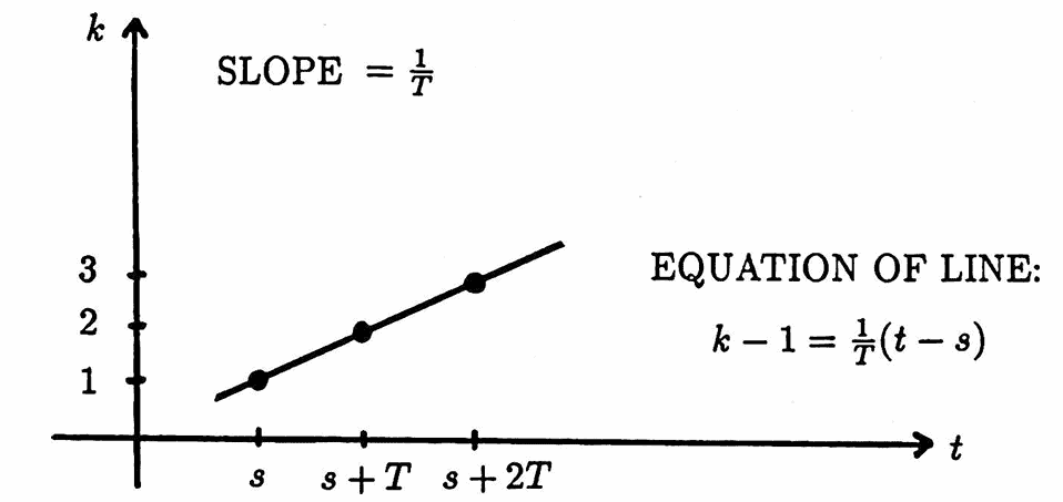
$$ t \mapsto \frac 1T(t-s) + 1 $$That is, the $i$th member of the initial time list maps to the positive integer $\,i\,.$
The symbol ‘$\,\mapsto\,$’ is read as ‘maps to’, and means that the element $\,t\,$ is sent to the element $\,\frac 1T(t-s) + 1\,.$
This transformation was found by writing down the equation of the line shown below:
It is equally easy to transform the list $\,(1,\,2,\,3,\,\ldots)\,$ back into a list with starting time $\,s\,,$ and uniform spacing $\,T\,.$ Indeed, the transformation
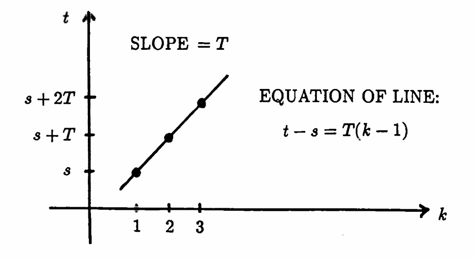
$$ k \mapsto T(k-1) + s $$maps the list
$$ (1,\ 2,\ 3,\,\ldots\,,\ i,\,\ldots\,, N,\,\ldots) $$to the list:
$$ \begin{align} &\bigl(s,\ s + T,\ s + 2T,\, \ldots\,,\cr\cr &\qquad s + (i-1)T, \, \ldots\,,\cr\cr &\qquad s + (N-1)T, \, \ldots\,\bigr) \end{align} $$This transformation was found by writing down the equation of the line shown below:
MATLAB commands for converting any finite uniform time list to the list $\,(1,2,3,\ldots,N)\,$; and for converting $\,(1,2,3,\ldots,N)\,$ back to a time list with starting value $\,s\,$ and spacing $\,T\,,$ are provided at the end of this section.
If an output list $\,(y_1,y_2,\ldots,y_N)\,$ corresponds to a uniform time list, then it has been shown that this associated time list can always be labeled $\,(1,2,3,\ldots,N)\,.$ Consequently, there is often no need to ‘carry around’ the associated time list. In such cases, the time list is often suppressed, and only the output list is given.
Functions are an extremely useful mathematical tool for working with input-output relationships that are characterized by each input having exactly one associated output. A convenient function notation that will be used throughout this dissertation is introduced next.
A function $\,f\,$ is a rule that associates to each input $\,x\,$ a unique output denoted by $\,f(x)\,.$
The set of inputs to $\,f\,$ is called the domain of $\,f\,$ and is denoted by $\,{\cal D}(f)\,.$
The notation
$$ f : {\cal D}(f) \to B $$symbolically indicates the rule $\,f\,,$ the domain $\,{\cal D}(f)\,,$ and a set $\,B\,$ that contains the outputs of $\,f\,.$ The set $\,B\,$ is called the codomain of $\,f\,.$
The actual output set of $\,f\,$ is called the range of $\,f\,$ and is denoted by $\,{\cal R}(f)\,.$ The range is found by letting $\,f\,$ act on all domain elements, and forming a set from the resulting function values; this action is sometimes indicated by:
$$ {\cal R}(f) = \{f(x)\ |\ x\in {\cal D}(f)\} $$In the notation $\,f : {\cal D}(f)\to B\,,$ it must be that $\,{\cal R}(f) \subset B\,.$
The set $\,B\,$ (the codomain of $\,f\,$) gives information about the type of outputs that the rule $\,f\,$ generates. The set $\,{\cal R}(f)\,$ gives information about the actual outputs that the rule $\,f\,$ generates.
For example, consider the function described by:
$$ f\, :\, \{x\ |\ 1 \le x\le 3\} \to \Bbb R\,,\ \ f(x) = x^2 $$Here, the fact that the codomain is $\,\Bbb R\,$ (where $\,R\,$ denotes the set of real numbers), implies that the outputs from $\,f\,$ are real numbers.
To find the range of $\,f\,,$ $\,{\cal R}(f)\,,$ one must see precisely what outputs are generated as the squaring function acts on all elements in the domain of $\,f\,$:
$$ \begin{align} {\cal R}(f) &= \{ f(x)\ |\ 1\le x\le 3\}\cr\cr &= \{ x^2\ |\ 1\le x\le 3\}\cr\cr &= \{ y\ |\ 1\le y\le 9\} \end{align} $$Note that the function notation $\,f : {\cal D}(f)\to B\,$ does not include information about how the outputs are related to the inputs. Such information must be provided separately.
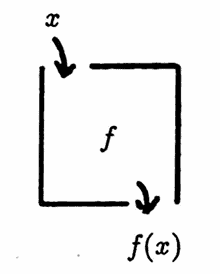
It is important to emphasize that $\,f\,$ is the name of the function; and $\,f(x)\,$ is the output of $\,f\,$ corresponding to the input $\,x\,.$
A function $\,f\,$ is called a discrete-domain function if its domain consists of entries from a time list.
Thus, the domain of a discrete-domain function is a set of time values (either finite or countably infinite), that can be listed in strictly increasing order.
In particular, a discrete-domain function has the property that its domain cannot contain any interval of real numbers.
Example: Using Function Notation
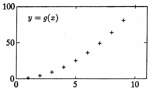
The function $\,f : [1,10]\to\Bbb R\,$ defined by $\,f(x) = x^2\,$ has the graph shown below. A related discrete-domain function $\,g : \{1,2,\ldots,10\}\to \Bbb R\,$ defined by $\,g(x) = x^2\,$ is also graphed.
Note that $\,{\cal R}(f) = [1,100]\,,$ and $\,{\cal R}(g) = \{1^2, 2^2, 3^2, \ldots , 10^2\}\,.$
![graph of the squaring function on the interval [1,10]](graphics/S1_2Img4.png)
In this dissertation, the codomain set will always be the real or complex numbers. If the codomain is $\,\Bbb R\,,$ then the function is called a real-valued function. If, in addition, the domain is a subset of $\,\Bbb R\,,$ then the function is called a real-valued function of a real variable.
Notation Used with Functions
The following notation is commonly used in connection with functions:
The symbol $\,\Bbb Z\,$ denotes the set of integers:
$$\Bbb Z := \{\ldots\,,{-}3,\,{-}2,\,{-}1,\,0,\,1,\,2,\,3,\,\ldots\}$$The symbol $\,\Bbb Z^+\,$ denotes the set of positive integers:
$$\Bbb Z^+ := \{1,\,2,\,3,\,\ldots\}$$More generally, the superscript ‘$\,+\,$’ always denotes the positive (strictly greater than zero) elements from a specified set.
The symbol $\,\Bbb Q\,$ denotes the set of rational numbers; i.e., the numbers that are expressible as a Quotient of integers (with nonzero denominator).
The symbol $\,\Bbb C\,$ denotes the set of complex numbers, i.e., those numbers that can be written in the form $\,a + bi\,,$ where $\,a\,$ and $\,b\,$ are real numbers, and $\,i := \sqrt{-1}\,.$ (Many engineers use $\,j\,$ to denote $\,\sqrt{-1}\,,$ since $\,i\,$ is reserved for electrical current.)
There is a convenient notation for intervals of real numbers. Let $\,a\,$ and $\,b\,$ be real numbers, with $\,a \lt b\,.$
An interval that does not include either endpoint, like
$$ (a,b) := \{x\ |\ a \lt x \lt b\} $$is called an open interval.
An interval that includes both endpoints, like
$$ [a,b] := \{x\ |\ a \le x \le b\} $$is called a closed interval.
An interval that includes exactly one endpoint, like
$$ \begin{gather} (a,b] := \{x\ |\ a \lt x \le b\}\cr \text{or}\cr [a,b) := \{x\ |\ a \le x \lt b\} \end{gather} $$is called a half-open interval.
Infinite intervals can be accommodated by using the symbol ‘$\,\infty\,$’ (‘infinity’), such as:
$$ [a,\infty) := \{x\ |\ x \ge a\} $$Observe that every discrete-domain data set $\,\{(t_i,y_i)\}_{i=1}^{(N\text{ or }\infty)}\,$ is naturally associated with a discrete-domain function $\,f\,$ that maps each input $\,t_i\,$ to the value $\,y_i\,,$ i.e., $\,f(t_i) = y_i\,.$
Thus, all discussions concerning discrete-domain data sets can be rephrased in terms of discrete-domain functions, if it is convenient to do so.
There are various phrases used in the existing literature that one should be aware of.
In communications and digital systems engineering, the phrase discrete signal usually refers to a data set associated with a function that has, as its domain, the entries from a time list. The codomain may be any subset of $\,\Bbb R\,.$
A digital signal is a special type of discrete signal, where not only the domain, but also the codomain, must consist of entries from a time list.
Thus, both discrete and digital signals are ‘sampled in time’. However, a discrete signal has the potential of taking on values in an interval; whereas a digital signal may only take its values from a time list. The difference is further clarified in the next example.
Example: Discrete Signal versus Digital Signal
The data set associated with a function
$$f : \{1,2,3\ldots\} \to [0,\infty)$$is a discrete signal, but not a digital signal, because $\,f\,$ has the potential of taking on values in an interval.
The data set associated with a function
$$g : \{1,2,3\ldots\} \to \{ 0,\ 0.01,\ 0.02,\ 0.03,\,\ldots\}$$is a digital signal, because $\,g\,$ only has the potential of taking on values from a time list.
In time series analysis and statistical literature, a time series is any list of observations generated sequentially in time, where there is thought to be a dependence between the observations and where the nature of this dependence is of interest.
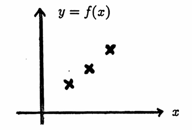
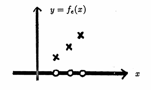
To conclude this section on notation, observe that any real-valued function $\,f\,$ defined on a proper subset of $\,\Bbb R\,$ can always be extended to a function $\,f_e\,$ defined on $\,\Bbb R\,,$ by defining $\,f_e\,$ to be zero for any input not in $\,{\cal D}(f)\,.$ That is, define:
$$ f_e(x) := \cases{ f(x) & \text{for } x\in {\cal D}(f)\cr\cr 0 & \text{for } x\notin {\cal D}(f) } $$Whenever the notation $\,f_e\,$ is used in this dissertation, it will denote this particular extension of a function $\,f\,$ to $\,\Bbb R\,.$
A function and its extension to $\,R\,$ are illustrated below.
MATLAB (‘MATrix LABoratory’) is a software package for numeric computation that has become quite popular in academia because of its powerful capabilities and ease of use. MATLAB commands will be used throughout this dissertation to implement the techniques discussed herein.
All MATLAB software given in this dissertation was created using PC-MATLAB for MS-DOS Personal Computer 286 users, Version 3.5k.
The reader is assumed to be a competent MATLAB user. However, as a convenience to the reader, the MATLAB commands used are reviewed on their first appearance. Examples are provided to illustrate the command sequences.
As I put this dissertation online (beginning December 2024), I tested all the original MATLAB code with GNU Octave. GNU Octave is free numeric computation software that is drop-in compatible with many MATLAB scripts.
I downloaded Version 9.2.0 of GNU Octave and used it on my Windows computer. The download came with both a command-line interface and a graphical-user interface.
Any changes or information needed for using Octave instead of MATLAB will be noted in a special-bordered box like this. If no such box appears, then all the given MATLAB commands should work—without any changes—in Octave.
MATLAB Implementation
Purpose
- To check that the time values in a data set are arranged in increasing order; if not, an appropriate rearrangement is made.
- To locate any repeated time values in a data set.
- To check for a uniform time list.
- To supply an alternative indexing of a uniform list: if the uniform list is of length$\,N\,,$ it can alternatively be indexed by $\,(1,\,\ldots\,, N)\,.$
-
To supply an alternative indexing of the list $\,(1,\,\ldots\,, N)\,$: if $\,s\,$ denotes a desired starting time and $\,T\,$ denotes a desired positive uniform spacing, then the alternative list
$$(s,\,s+T,\,\ldots\,, s + (N-1)T)$$is produced.
Required Inputs
The data set being investigated must be contained in an $\,N \times 2\,$ matrix, denoted here by z . The first column of z contains the time values; the second column contains the corresponding outputs.
| z = | ||
| t1 | y1 | |
| t2 | y2 | |
| t3 | y3 | |
| $\ \vdots$ | $\ \vdots$ | |
| tN | yN |
The positive integer $\,N\,$ denotes the number of ordered pairs in the data set.
MATLAB Commands
The commands listed below are used to re-order the ordered pairs, so that the resulting time values are in increasing order. The resulting (re-ordered) matrix replaces the original matrix.
Then, locations of any repeated time values in the re-ordered matrix are given.
The lines are numbered for easy reference in the discussion that follows.
1)  t = z(:,1);
2)  y = z(:,2);
3)  [t,i] = sort(t);
4)  y = y(i);
5)  z = [t y];
6)  for j = 1:(length(t)-1),
7)    if t(j) == t(j+1),
8)      j
9)    end
10) end
Line 1: The first column of z is named t . The colon operator ‘:’ is used here to denote all the rows of the matrix z . The semicolon ‘;’ at the end of the line suppresses MATLAB echoing.
Line 2: The second column of z is named y .
Line 3: The entries of t are sorted in ascending order; the resulting column vector is again denoted by t . The list i contains the re-ordering information, and is used next to correspondingly re-order the entries in y .
Line 4: The entries in y are re-arranged to coincide with the new arrangement in t . This re-arrangement of y is again denoted by y .
Line 5: The original matrix z is replaced by the re-ordered matrix.
Lines 6–10: If entries j and j+1 of the (re-ordered) list t are identical, then the value j is returned. The analyst can then make appropriate adjustments to the data set.
If desired, lines 6–10 could be stored in an m-file, say, chkfdup.m (check for duplicates). Then, lines 6–10 would be replaced by the single command, chkfdup .
In order for Octave to find your scripts, you may need to add a search path using the Octave command addpath() .
For example, the Octave command
addpath('C:\Users\carol\Desktop\Scripts')
enables Octave to locate scripts (like chkfdup ) that are stored in the Scripts folder on my desktop.
Continuing the commands above, the adjusted list t is checked, to see if it is a uniform time list. If not, the positions of ‘errant’ time values are returned in the list err .
11) d = diff(t);
12) p = ( ones(d)*d(1) ~= d );
13) err = find(p);
p = ( ones(size(d))*d(1) ~= d );
Newer versions of MATLAB may also need this revised code.Line 11
The vector d contains the successive differences of the entries in t . That is:
d(1) = t2 - t1
d(2) = t3 - t2
$\vdots$
If t is uniform, then all the entries in d are identical; and if all the entries in d are identical, then t is uniform.
Line 12
The list ones(d)*d(1) has the same size as d , with all entries equal to d(1) . Instead of d(1) , the analyst may choose to use d(j) for values of j greater than 1 .
Via the command ‘( ones(d)*d(1) ~= d )’ the list ones(d)*d(1) is compared to the list d .
If the relation ‘( ones(d)*d(1) ~= d )’ is TRUE, then a value of ‘1’ is returned in the list p . At these positions, a spacing different than the spacing between t2 and t1 is encountered.
If the relation ‘( ones(d)*d(1) ~= d )’ is FALSE, then a value of ‘0’ is returned in the list p .
Line 13
The MATLAB command ‘find’ locates the nonzero entries in a matrix. Each entry in p is either ‘1’ or ‘0’ ; therefore, the locations of the ‘1’ entries in p are recorded in err .
Alternative indexing
The command
(1:length(t))';
produces a vertical list of the positive integers 1,2,3,...,N , where N = length(t) .
Given a list t = (1,2,3,...,N) , the command
resp_t = (s : T : s+(length(t)-1)*T )';
% ‘resp’ is for ‘respace’
produces a vertical list of length N , starting at s and with uniform spacing T .
Example
The following diary of an actual MATLAB session illustrates the command sequences just discussed.
z = [.5 11; 2 14; 1 12.1; 1.5 12.9; 0 10; 1 12; 2.4 14.9; 3 16]
z =
    0.5000   11.0000
    2.0000   14.0000
    1.0000   12.1000
    1.5000   12.9000
         0   10.0000
    1.0000   12.0000
    2.4000   14.9000
    3.0000   16.0000
t = z(:,1);
y = z(:,2);
[t,i] = sort(t)
t =
         0
    0.5000
    1.0000
    1.0000
    1.5000
    2.0000
    2.4000
    3.0000

i =
    5
    1
    3
    6
    4
    2
    7
    8
y = y(i);
z = [t y]
z =
         0  10.0000
    0.5000  11.0000
    1.0000  12.1000
    1.0000  12.0000
    1.5000  12.9000
    2.0000  14.0000
    2.4000  14.9000
    3.0000  16.0000
chkfdup
j =
    3
% the analyst decides to delete row 3 of z
z(3,:) = [];
% let t be the first column
% of the adjusted data set
t = z(:,1);
d = diff(t)
d =
    0.5000
    0.5000
    0.5000
    0.5000
    0.4000
    0.6000
p = ( ones(d)*d(1) ~= d)
p =
    0
    0
    0
    0
    1
    1
err = find(p)
err =
    5
    6
% the analyst observes non-uniform spacing
% in lines 5-6, and 6-7 of z
% re-index t with positive integers
tnew = (l:length(t))'
tnew =
    1
    2
    3
    4
    5
    6
    7
% reindex tnew with s = 0, T = .5
tnew = (0:.5:0+(length(tnew)-1)*(.5))'
tnew =
         0
    0.5000
    1.0000
    1.5000
    2.0000
    2.5000
    3.0000