2.3 Computer Application Considerations for Linear Least-Squares
Condition Numbers
In the previous section, it was shown that the problem
$$ \underset{\,\boldsymbol{\rm b} \in \Bbb R^n}{\text{min}}\ \|\boldsymbol{\rm y} - \boldsymbol{\rm Xb}\|^2 $$has a unique solution, provided that the square matrix $\,\boldsymbol{\rm X}^t\boldsymbol{\rm X}\,$ is invertible.
Theoretically (using exact arithmetic), the invertibility of a square matrix $\,A\,$ is easily characterized in a variety of ways: for example, $\,A\,$ is invertible if and only if the determinant of $\,A\,$ (denoted by $\,\text{det}(A)\,$) is nonzero, and in this case, the unique solution to $\,Ax = b\,$ is given by $\,x = A^{-1}b\,.$
However, when the entries of a matrix are represented only to the degree of accuracy of a digital computer, the question of invertibility is more subtle: there are invertible matrices $\,A\,$ for which correct numerical solutions to $\,Ax = b\,$ are difficult to obtain, stemming from the fact that small changes in the matrices $\,A\,$ and $\,b\,$ can lead to large changes in the solution $\,x\,.$
Example: MATLAB Casts Suspicion on a Solution Vector
To illustrate this point, reconsider the MATLAB example of the previous section, where a $4^{\text{th}}$-order polynomial least-squares approximate of the data
$$ y(t) = 3.2 - 0.7t + 0.05t^2 + \sin\frac{2\pi t}3 + \langle\text{noise}\rangle $$was found. If, alternatively, a $7^{\text{th}}$-order polynomial approximate was sought, the MATLAB user would have been faced with this warning, casting suspicion on the resulting vector $\,\boldsymbol{\rm b}\,$:
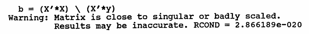
The size of $\,\boldsymbol{\rm X}^t\boldsymbol{\rm X}\,$ is only $\,8\times8\,$; however, the entries of $\,\boldsymbol{\rm X}^t\boldsymbol{\rm X}\,$ are such that the matrix does not lend itself nicely to numerical computation. This problem is the subject of the current section.
More precisely, this section gives an analysis of the system $\,Ax = b\,$ in order to understand the sensitivity of solutions $\,x\,$ to small changes in the matrices $\,A\,$ and $\,b\,.$ A number $\,\text{cond}(A)\,$ will be defined that measures this sensitivity.
For a ‘sensitive’ system, correct numerical solution can be challenging, but the problem can often be overcome by replacing the system $\,Ax = b\,$ with an equivalent system $\,\tilde Ax = b\,,$ where the new matrix $\,\tilde A\,$ is more suitable for numerical computations. This replacement requires a knowledge of discrete orthogonal functions, which are also discussed in this section.
Let $\,\phi\, :\, X\rightarrow Y\,$ be a function between normed spaces. The reader is referred to Appendix 2 for a review of normed spaces. The symbol $\,\|\cdot\|\,$ will be used to denote both the $\,X\,$ and $\,Y\,$ norms, with context determining the correct interpretation.
Let $\,x\in X\,,$ and let $\,\tilde x\,$ be an approximation to $\,x\,.$ For $\,x \ne 0\,,$ the relative error of $\,\tilde x\,$ (as an approximation to $\,x\,$) is defined to be the number:
$$ \frac{\|\tilde x - x\|}{\|x\|} $$Similarly, for $\,\phi(x)\ne 0\,,$ the relative error of $\,\phi(\tilde x)\,$ (as an approximation to $\,\phi(x)\,$) is the number:
$$ \frac{\|\phi(\tilde x) - \phi(x)\|}{\|\phi(x)\|} $$A desirable situation for the function $\,\phi\,$ is this: when the relative error in $\,\tilde x\,$ is small, so is the relative error in $\,\phi(\tilde x)\,.$ In other words, small input errors lead to small output errors. To quantify this input/output relationship, the idea of a condition number is introduced:
Let $\,\phi\ :\ X\rightarrow Y\,$ be a function between normed spaces, and let $\,x\in X\,.$ If a real number $\,c \gt 0\,$ exists for which
$$ \frac{\|\phi(\tilde x) - \phi(x)\|}{\|\phi(x)\|} \le c\,\frac{\|\tilde x - x\|}{\|x\|} $$for all $\,\tilde x\,$ sufficiently close to $\,x\,,$ then $\,c\,$ is called a condition number for $\,\phi\,$ at $\,x\,.$
This definition shows that $\,c\,$ gives information about the amplification of relative input errors. If $\,c\,$ is small, then small input errors must produce small output errors. However, if $\,c\,$ is large, or if no such positive number $\,c\,$ exists, then small input errors may produce large output errors.
In numerical problems, where numbers often inherently contain error (due to a forced finite computer representation), such considerations become important.
Note that the definition of condition number is dependent on both the norm in the domain $\,X\,,$ and the norm in the codomain $\,Y\,.$
For an invertible matrix $\,A\,,$ the system $\,Ax = b\,$ will be analyzed as follows: the matrices $\,A\,$ and $\,b\,$ are taken as the ‘inputs’ to the system, and a solution vector $\,x\,$ is the ‘output’.
When the inputs $\,A\,$ and $\,b\,$ change slightly (say, by replacing theoretical matrices $\,A\,$ and $\,b\,$ by their computer representations), then it is desired to study how the solution $\,x\,$ changes.
The Euclidean norm $\,\|\cdot\|\,$ will be used to measure ‘changes’ in the $\,n \times 1\,$ matrix $\,b\,.$ It is also necessary to have a means by which to measure changes in the matrix $\,A\,$; this means will be provided by a matrix norm, defined next. In this next definition, $\,\text{sup}\,$ denotes the supremum, i.e., the least upper bound.
Let $\,A\,$ be any $\,n \times n\,$ matrix, and let $\,\|\cdot\|$ be the Euclidean norm on $\,\Bbb R^n\,.$ The $2$-norm of the matrix $\,A\,$ is given by:
$$ \|A\|_2 := \underset{\substack{x\in\Bbb R^n\,,\cr x\ne 0}} {\text{sup}} \frac{\|Ax\|}{\|x\|} $$It can be shown that the $2$-norm is indeed a norm on the vector space of all $\,n\times n\,$ matrices. Consequently, if $\,\|A\|_2 = 0\,,$ then $\,A = \boldsymbol{0}\,,$ where $\,\boldsymbol{0}\,$ denotes the $\,n \times n\,$ zero matrix. Thus, if $\,\|A\|_2 = 0\,,$ then $\,A\,$ is not invertible. Equivalently, if $\,A\,$ is invertible, then $ \,\|A\|_2 \ne 0\,.$
The number $\|A\|_2\,$ is approximated in MATLAB via the command:
norm(A)
There are other matrix norms (see, e.g., [S&B, p. 178]), many of which are more easily calculated than $\,\|\cdot\|_2\,,$ but it will be seen that the $2$-norm is particularly well suited to the current situation.
The reader versed in functional analysis will recognize the $2$-norm as the norm of the bounded linear operator $\,A: \Bbb R^n\rightarrow \Bbb R^n\,,$ when the Euclidean norm is used in $\,\Bbb R^n\,.$
It is immediate from the definition of $\,\|A\|_2\,$ that for any $\,x\ne 0\,,$
$$ \|A\|_2 \ge \frac{\|Ax\|}{\|x\|}\,, $$so that for all $\,x\,$:
$$ \|Ax\| \le \|A\|_2\cdot \|x\| \tag{1} $$Thus, the number $\|A\|_2\,$ gives the greatest magnification that a vector may attain under the mapping determined by $\,A\,.$ That is, the norm of an output $\,\|Ax\|\,$ cannot exceed $\,\|A\|_2\,$ times the norm of the corresponding input $\,\|x\|\,.$
The $2$-norm is not easy to compute. ($\bigstar$ When $\,A\,$ has real number entries, $\|A\|_2\,$ is the square root of the largest eigenvalue of the matrix $\,A^tA\,.$) However, it is easy to obtain an upper bound for $\,\|A\|_2\,$ as the square root of the sum of the squared entries from $\,A\,,$ as follows:
Let $\,x = (x_1,\ldots,x_n)^t\,,$ so that $\,x\,$ is a column vector, and:
$$ \|x\| = \left( \sum_{i=1}^n x_i^2 \right)^{1/2} $$Let $\,\alpha_{ij}\,$ denote the element in row $\,i\,$ and column $\,j\,$ of the matrix $\,A\,.$ The $\,i^{\text{th}}\,$ component of the column vector $\,Ax\,$ is denoted by $\,(Ax)_i\,,$ and is the inner product of the $\,i^{\text{th}}\,$ row of $\,A\,$ with $\,x\,$:
$$ (Ax)_i = \sum_{j=1}^n \alpha_{ij}x_j $$Then:
$$ \begin{align} \|Ax\|^2 &=\sum_{i=1}^n (Ax)_i^2 = \sum_{i=1}^n \left( \sum_{j=1}^n \alpha_{ij}x_j \right)^2\cr\cr &\le \sum_{i=1}^n \left[ \left( \sum_{j=1}^n \alpha_{ij}^2 \right)^{1/2} \left( \sum_{j=1}^n x_j^2 \right)^{1/2} \right]^2\cr &\qquad \text{(Cauchy-Schwarz)}\cr\cr &= \|x\|^2 \sum_{i=1}^n\sum_{j=1}^n \alpha_{ij}^2 \end{align} $$(The Cauchy-Schwarz Inequality is reviewed in Appendix $2\,.$)
Thus, for any $\,x\ne 0\,,$ division by $\,\|x\|^2\,$ yields
$$ \frac{\|Ax\|^2}{\|x\|^2} \le \sum_{i=1}^n\sum_{j=1}^n \alpha_{ij}^2\ , $$so that taking square roots gives:
$$ \begin{align} \|A\|_2 &:= \underset{\substack{x\in\Bbb R^n\cr x\ne 0}}{\text{sup}} \frac{\|Ax\|}{\|x\|}\cr\cr &\le \left( \sum_{i=1}^n \sum_{j=1}^n \alpha_{ij}^2 \right)^{1/2}\cr\cr &:= \|A\|_F \end{align} $$The square root of the sum of the squared entries from $\,A\,$ gives another norm of $\,A\,,$ called the Frobenius norm, and denoted by $\,\|A\|_F\,$ [G&VL, p. 56].
Many of the ideas discussed in this section are conveniently expressed in terms of the singular values of $\,A\,.$ In particular, the norms $\,\|A\|_2\,$ and $\,\|A\|_F\,$ have simple characterizations in terms of the singular values.
The singular value decomposition of a matrix is discussed in Appendix $2\,.$
With the matrix $2$-norm in hand, the analysis of the system $\,Ax = b\,$ can now begin. It is assumed that $\,A\,$ is an invertible $\,n \times n\,$ matrix with real number entries. It is desired to study the sensitivity of solutions $\,x\,$ of this system to small changes in $\,A\,$ and $\,b\,.$
[S&B, 178–180] Begin by supposing that only the column vector $\,b\,$ changes slightly; $\,A\,$ remains fixed. What is the corresponding effect on the solution $\,x\,$? The analysis of this situation will motivate the definition of the condition number of a matrix.
Let
$$ \begin{gather} Ax = b\cr \text{and}\cr A\tilde x = \tilde b \end{gather} $$be true statements; that is, $\,x\,$ denotes the system solution when column vector $\,b\,$ is used, and $\,\tilde x\,$ denotes the system solution when column vector $\,\tilde b\,$ is used. Define
$$ \begin{gather} \Delta x := \tilde x - x\cr \text{and}\cr \Delta b := \tilde b - b\ , \end{gather} $$so that:
$$ A\Delta x = \Delta b $$Since $\,A\,$ is invertible (by hypothesis):
$$ \Delta x = A^{-1}\Delta b $$Taking norms and using property ($1$) gives:
$$ \begin{align} \|\Delta x\| &= \|A^{-1}\Delta b\|\cr\cr &\le \|A^{-1}\|_2\cdot \|\Delta b\| \end{align} $$Let $\,x\ne 0\,$; division by the positive number $\,\|x\|\,$ gives:
$$ \frac{\|\Delta x\|}{\|x\|} \le \frac{\|A^{-1}\|_2\cdot \|\Delta b\|}{\|x\|} $$Since $\,b = Ax\,,$ it follows that $\,\|b\| \le \|A\|_2\cdot\|x\|\,$ and hence $\,\frac1{\|x\|} \le \frac{\|A\|_2}{\|b\|}\,$; substitution into the previous display yields:
$$ \frac{\|\Delta x\|}{\|x\|} \le \|A^{-1}\|_2\ \|A\|_2\ \frac{\|\Delta b\|}{\|b\|} $$This inequality shows that the constant $\,\|A^{-1}\|_2\,\|A\|_2\,$ gives information about how an error in $\,b\,$ is potentially ‘amplified’ to produce an error in the solution $\,x\,$.
Thus, the number $\,\|A^{-1}\|_2\,\|A\|_2\,$ is a condition number for the function that ‘inputs’ a column vector $\,b\,,$ and ‘outputs’ a solution to the system $\,Ax = b\,.$ With this motivation, the next definition should come as no surprise:
Let $\,A\,$ be an invertible matrix. The condition number of $\,A\,$ is:
$$ \text{cond}(A) := \|A^{-1}\|_2\cdot\|A\|_2 $$The condition number $\,\text{cond}(A)\,$ is approximated in MATLAB via the command:
cond(A)
When $\,\text{cond}(A)\,$ is close to $\,1\,,$ $\,A\,$ is said to be well-conditioned, and when $\,\text{cond}(A)\,$ is large, $\,A\,$ is said to be ill-conditioned.
It is always true that $\,\text{cond}(A) \ge 1\,,$ as follows. Since $\,\|A\|_2\ge\frac{\|Ay\|}{\|y\|}\,$ for all $\,y\ne 0\,,$ take $\,y\,$ to be $\,A^{-1}x\,,$ thus obtaining
$$ \begin{align} \|A\|_2 &\ge \frac{\|A(A^{-1}x)\|}{\|A^{-1}x\|}\cr\cr &= \frac{\|x\|}{\|A^{-1}x\|}\cr\cr &\ge \frac{\|x\|}{\|A^{-1}\|_2\,\|x\|}\ , \end{align} $$from which:
$$ \begin{align} \|A\|_2\,\|A^{-1}\|_2 &\ge\frac{\|x\|}{\|A^{-1}\|_2\,\|x\|}\cdot\|A^{-1}\|_2\cr\cr &= 1 \end{align} $$If $\,A\,$ is an orthogonal matrix (that is, $\,A^t A = I\,,$ or equivalently, $\,A^{-1} = A^t\,$), then it can be shown that $\,\text{cond}(A) = 1\,.$
When MATLAB issues warnings regarding ill-conditioned matrices, it reports the information in terms of the reciprocal of the condition number:
rcond(A) := 1/(cond(A))
If $\,A\,$ is well-conditioned, then rcond(A) is near $\,1.0\,$; if $\,A\,$ is ill-conditioned, then rcond(A) is near $\,0\,.$
It is important to note that, in the system $\,Ax=b\,,$ the sensitivity of solutions $\,x\,$ to small changes in $\,b\,$ clearly has more to do with $\,A\,$ than with $\,b\,.$
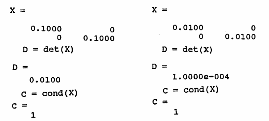
Since $\,A\,$ is invertible if and only if $\,\text{det}(A) \ne 0\,,$ one might conjecture that when the determinant of $\,A\,$ is close to $\,0\,,$ then solutions to $\,Ax = b\,$ are sensitive to small changes in $\,A\,.$ However, this is not the case. The examples below show that $\,\text{det}(A)\,$ can be made as small as desired, while keeping $\,\text{cond}(A) = 1\,.$
The definition of the condition number of a matrix was motivated by studying the sensitivity of solutions to $\,Ax = b\,$ to small changes in $\,b\,.$ Does the number $\,\text{cond}(A)\,,$ as defined, also measure the sensitivity of solutions to changes in both $\,A\,$ and $\,b\,$? The following discussion shows that the answer is ‘Yes’.
[G&VL, 79–80] Allow both $\,A\,$ and $\,b\,$ to vary in the system $\,Ax = b\,$; recall that $\,A\,$ is assumed to be invertible.
Denote a change in $\,A\,$ by $\,\epsilon F\,,$ where $\,F\,$ is an $\,n \times n\,$ constant matrix and $\epsilon\gt 0\,.$ Similarly, denote a change in $\,b\,$ by $\,\epsilon f\,,$ where $\,f\,$ is a fixed $\,n \times 1\,$ matrix. Different values of $\,\epsilon\,$ lead to different approximations $\,\tilde A := A + \epsilon F\,$ and $\,\tilde b := b + \epsilon f\,$ of $\,A\,$ and $\,b\,,$ respectively.
Let $\,x(\epsilon)\,$ denote the solution of the ‘perturbed’ system $\,\tilde Ax = \tilde b\,$; the situation is then summarized by:
$$ (A + \epsilon F)\,x(\epsilon) = b + \epsilon f\,,\ \ x(0) = x $$Differentiating both sides with respect to $\,\epsilon\,$ yields:
$$ (A + \epsilon F)\,\dot x(\epsilon) + F\,x(\epsilon) = f $$Evaluation at $\,\epsilon = 0\,$ and a slight rearrangement yields:
$$ A\,\dot x(0) = f - Fx $$Or, since $\,A\,$ is invertible:
$$ \dot x(0) = A^{-1}(f-Fx) \tag{2} $$The Taylor expansion for $\,x\,$ (as a function of the single variable $\,\epsilon\,$) is:
$$ x(\epsilon) = x + \epsilon\,\dot x(0) + \overbrace{\frac{\ddot x(0)}{2!}\epsilon^2 + \frac{\dddot x(0)}{3!}\epsilon^3 + \cdots}^{o(\epsilon)} $$The notation $\,o(\epsilon)\,$ is used to represent the fact that the indicated terms converge to $\,0\,$ faster than $\,\epsilon\,$ converges to $\,0\,$; that is:
$$ \lim_{\epsilon\rightarrow 0} \frac{ \frac{\ddot x(0)}{2!}\epsilon^2 + \frac{\dddot x(0)}{3!}\epsilon^3 + \cdots}{\epsilon} = 0 $$Thus, when $\,\epsilon\,$ is close to $\,0\,,$ the power series is well-approximated by its first two terms.
Substitution of formula $(2)$ for $\,\dot x(0)\,$ into the approximate equation $\,x(\epsilon) = x + \epsilon\,\dot x(0)\,$ gives the approximate equation:
$$ x(\epsilon) = x + \epsilon A^{-1}(f - Fx) $$Rearranging and taking norms yields:
$$ \begin{align} \|x(\epsilon) - x\| &= \|\epsilon A^{-1}(f - Fx)\|\cr\cr &\le \epsilon\,\|A^{-1}\|_2\, \|f - Fx\| \end{align} $$Division by $\,\|x\|\,$ and rearrangement gives:
$$ \begin{align} \frac{\|x(\epsilon) - x\|}{\|x\|} &\le \epsilon\,\|A^{-1}\|_2\, \frac{\|f - Fx\|}{\|x\|}\cr\cr &\le \epsilon\,\|A^{-1}\|_2\, \frac{\|f\| + \|F\|_2\,\|x\|}{\|x\|}\cr\cr &= \|A^{-1}\|_2 \left( \epsilon\frac{\|f\|}{\|x\|} + \epsilon\,\|F\|_2 \right)\cr\cr &= \|A^{-1}\|_2\,\|A\|_2 \left( \epsilon\,\frac{\|f\|}{\|A\|_2\,\|x\|} + \epsilon\,\frac{\|F\|_2}{\|A\|_2} \right)\cr\cr &= \text{cond}(A) \left( \frac{\|\epsilon f\|}{\|A\|_2\,\|x\|} + \frac{\|\epsilon F\|_2}{\|A\|_2} \right)\cr\cr &\le \text{cond}(A) \left( \frac{\|\epsilon f\|}{\|b\|} + \frac{\|\epsilon F\|_2}{\|A\|_2} \right) \end{align} $$Recalling that $\,\epsilon f\,$ and $\,\epsilon F\,$ denote changes in $\,b\,$ and $\,A\,,$ respectively, this final form shows that the condition number of $\,A\,$ does indeed measure the sensitivity of solutions to changes in the initial data $\,A\,$ and $\,b\,.$
Discrete Orthogonal Functions
Next, the concept of discrete orthogonal functions, and MATLAB implementation of these ideas, is introduced as a way of dealing with sensitive systems that may arise from linear least-squares approximation.
The reader is referred to Appendix $2$ for a review of the linear algebra concepts (e.g., inner products, orthogonal vectors, Gram-Schmidt process) that appear in this section.
If MATLAB balks in a solution attempt of the linear least-squares problem
$$ \underset{\boldsymbol{\rm b}\in\Bbb R^n}{\text{min}}\ \|\boldsymbol{\rm y} - \boldsymbol{\rm X}\boldsymbol{\rm b}\|^2\ , \tag{3} $$because the condition number of $\,\boldsymbol{\rm X}^t\boldsymbol{\rm X}\,$ is too large, then what can be done? One solution is to transform the set of modeling functions $\,f_1,f_2,\ldots,f_m\,$ into a replacement set $\,F_1,F_2,\ldots,F_m\,,$ that has the following properties:
-
Any function representable as a linear combination of the $\,f_i\,$ is also representable as a linear combination of the $\,F_i\,$ (and vice versa). That is:
$$ \begin{align} &\{c_1f_1 + \cdots + c_mf_m\ |\ c_i\in\Bbb R\}\cr &\quad = \{c_1F_1 + \cdots + c_mF_m\ |\ c_i\in\Bbb R\}\cr \end{align} $$ - The matrix $\,\boldsymbol{\rm \tilde X}^t\boldsymbol{\rm\tilde X}\,$ that results from using the functions $\,F_i\,$ is much better suited to numerical computations than the matrix $\,\boldsymbol{\rm X}^t\boldsymbol{\rm X}\,$ that uses the original $\,f_i\,.$
The new functions $\,F_i\,$ will be linear combinations of the original functions $\,f_i\,,$ and consequently will usually be considerably more complicated than the original $\,f_i\,.$
For a matrix $\,\boldsymbol{\rm A},$ the notation $\,\boldsymbol{\rm A}_{ij}\,$ is used to denote the entry in row $\,i\,$ and column $\,j\,$ of $\,{\boldsymbol{\rm A}}\,.$
Recall that the matrix $\,\boldsymbol{\rm X}\,$ in the linear least-squares problem $(3)$ is constructed by setting
$$ \boldsymbol{\rm X}_{ij} = f_j(t_i)\ , $$where $\,f_i\,$ ($\,i = 1,\ldots,m\,$) are the modeling functions, and $\,t_i\,$ ($\,i = 1,\ldots,N\,$) are the time values of the data points (see Section 2.2).
Therefore, $\,\boldsymbol{\rm X}_{ij}^t = \boldsymbol{\rm X}_{ji} = f_i(t_j)\,.$ The $\,ij^{\text{th}}$ entry of $\,\boldsymbol{\rm X}^t\boldsymbol{\rm X}\,$ is found by taking the inner product of the $\,i^{\text{th}}\,$ row of $\,\boldsymbol{\rm X}^t\,$ with the $\,j^{\text{th}}\,$ column of $\,\boldsymbol{\rm X}\,,$ yielding:
$$ \begin{align} (\boldsymbol{\rm X}^t\boldsymbol{\rm X})_{ij} &=\sum_{k=1}^N \boldsymbol{\rm X}_{ik}^t\boldsymbol{\rm X}_{kj}\cr\cr &= \sum_{k=1}^N f_i(t_k)\,f_j(t_k) \tag{4} \end{align} $$If the matrix $\,\boldsymbol{\rm X}^t\boldsymbol{\rm X}\,$ is diagonal, then the system $\,\boldsymbol{\rm X}^t\boldsymbol{\rm X}\boldsymbol{\rm b} = \boldsymbol{\rm X}^t\boldsymbol{\rm y}\,$ is trivial to solve for $\,\boldsymbol{\rm b}\,.$ From (4), it is clear that $\,\boldsymbol{\rm X}^t\boldsymbol{\rm X}\,$ is diagonal if and only if:
$$ \begin{gather} \sum_{k=1}^N f_i(t_k)f_j(t_k) = 0\cr \text{for all}\ \ i\ne j\,,\ \ i,j = 1,\ldots,m \end{gather} $$Functions $\,f_i\,$ and time values $\,t_i\,$ that satisfy such a condition are therefore particularly desirable. This idea is captured in the following definition:
Let $\,f_1,\ldots,f_m\,$ be real-valued functions of one real variable, and let $\,t_1,\ldots,t_N\,$ be $\,N\,$ distinct real numbers.
The functions $\,f_1,\ldots,f_m\,$ are mutually orthogonal with respect to the time values $\,t_1,\ldots,t_N\,$ if:
$$ \begin{gather} \sum_{k=1}^N f_i(t_k)f_j(t_k) = 0\cr \text{for all}\ \ i\ne j\,,\ \ i,j = 1,\ldots,m \end{gather} $$Functions $\{f_i\}_{i=1}^m\,$ satisfying this property are informally referred to as discrete orthogonal functions.
For vectors $\,\boldsymbol{\rm u} := (u_1,\ldots,u_N)\,$ and $\,\boldsymbol{\rm v} := (v_1,\ldots,v_N)\,$ in $\,\Bbb R^N\,,$ the notation $\langle\boldsymbol{\rm u},\boldsymbol{\rm v}\rangle$ denotes the Euclidean inner product of $\,\boldsymbol{\rm u}\,$ and $\,\boldsymbol{\rm v}\,$:
$$ \langle\boldsymbol{\rm u},\boldsymbol{\rm v}\rangle = \sum_{k=1}^N u_kv_k $$Vectors $\,\boldsymbol{\rm u}\,$ and $\,\boldsymbol{\rm v}\,$ are orthogonal if and only if $\,\langle\boldsymbol{\rm u},\boldsymbol{\rm v}\rangle = 0\,.$
Let $\,\boldsymbol{\rm T} = (t_1,\ldots,t_N)\,$ be an $N$-tuple of distinct time values, and let $\,f\,$ be a real-valued function of one real variable. The notation $\boldsymbol{\rm f}(\boldsymbol{\rm T})\,$ denotes the $N$-tuple:
$$ \boldsymbol{\rm f}(\boldsymbol{\rm T}) := \bigl( f(t_1),\ldots,f(t_N) \bigr) $$If $\,\boldsymbol{\rm T}\,$ is understood from context, then $\boldsymbol{\rm f}(\boldsymbol{\rm T})\,$ is more simply written as $\,\boldsymbol{\rm f}\,.$
In particular, a function $\,f_i\,$ has associated $N$-tuple:
$$ \boldsymbol{\rm f}_i := \bigl( f_i(t_1),\ldots,f_i(t_N) \bigr) $$With the notation above, functions $\,f_1,\ldots,f_m\,$ are mutually orthogonal with respect to time values $\,\boldsymbol{\rm T} = (t_1,\ldots,t_N)\,$ if and only if $\,\boldsymbol{\rm f}_i\,$ is orthogonal to $\,\boldsymbol{\rm f}_j\,,$ whenever $\,i\ne j\,.$
In a typical linear least-squares application, the number of approximating functions ($\,m\,$) is much less than the number of time values ($\,N\,$). In this case, the $\,m\,$ vectors $\,\boldsymbol{\rm f}_1,\ldots,\boldsymbol{\rm f}_m\,$ span a finite-dimensional subspace of $\,\Bbb R^N\,.$
If the vectors $\,\boldsymbol{\rm f}_1,\ldots,\boldsymbol{\rm f}_m\,$ are linearly independent, then they span an $m$-dimensional subspace of $\,\Bbb R^N\,.$ In this case, the Gram-Schmidt orthogonalization procedure can be used to replace the original vectors $\,\boldsymbol{\rm f}_i\,$ by new vectors $\,\boldsymbol{\rm F}_i\,$ that are mutually orthogonal in $\,\Bbb R^N\,,$ and that span precisely the same subspace of $\,\Bbb R^N\,.$
Correspondingly, the original functions $\,f_i\,$ are replaced by new functions $\,F_i\,$ that are mutually orthogonal with respect to $\,\boldsymbol{\rm T}\,.$ This procedure is illustrated in the next example.
Example
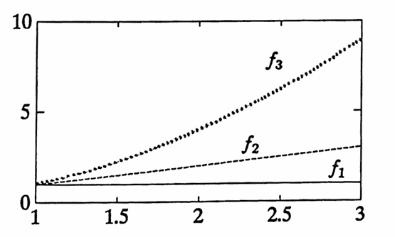
Let
$$ f_1(t) = 1\,,\ \ f_2(t) = t\,,\ \ f_3(t) = t^2\,, $$and let:
$$ \boldsymbol{\rm T} = (1,2,3) $$Then:
$$ \begin{gather} \boldsymbol{\rm f}_1 = (1,1,1)\,,\cr \boldsymbol{\rm f}_2 = (1,2,3)\,,\cr \text{and}\cr \boldsymbol{\rm f}_3 = (1,4,9) \end{gather} $$The Gram-Schmidt process yields:
$$ \begin{align} \boldsymbol{\rm F}_1 &= \frac{\boldsymbol{\rm f}_1}{\|\boldsymbol{\rm f}_1\|} = \frac 1{\sqrt 3}(1,1,1)\ ,\cr\cr \boldsymbol{\rm F}_2 &= \frac{\boldsymbol{\rm f}_2 - \langle\boldsymbol{\rm f}_2,\boldsymbol{\rm F}_1\rangle \boldsymbol{\rm F}_1 } {\|\boldsymbol{\rm f}_2 - \langle\boldsymbol{\rm f}_2,\boldsymbol{\rm F}_1\rangle \boldsymbol{\rm F}_1 \|}\cr &= \cdots = \frac 1{\sqrt 2}(-1,0,1)\ ,\ \ \text{and}\cr\cr \boldsymbol{\rm F}_3 &= \frac{\boldsymbol{\rm f}_3 - \langle\boldsymbol{\rm f}_3,\boldsymbol{\rm F}_1\rangle \boldsymbol{\rm F}_1 - \langle\boldsymbol{\rm f}_3,\boldsymbol{\rm F}_2\rangle \boldsymbol{\rm F}_2 } {\|\boldsymbol{\rm f}_3 - \langle\boldsymbol{\rm f}_3,\boldsymbol{\rm F}_1\rangle \boldsymbol{\rm F}_1 - \langle\boldsymbol{\rm f}_3,\boldsymbol{\rm F}_2\rangle \boldsymbol{\rm F}_2 \|}\cr &= \cdots = \frac 1{\sqrt 6}(1,-2,1) \end{align} $$It is routine to check that the $\,\boldsymbol{\rm F}_i\,$ are mutually orthogonal in $\,\Bbb R^3\,.$
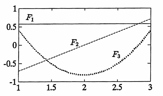
By writing the $\,\boldsymbol{\rm F}_i\,$ as linear combinations of the $\,\boldsymbol{\rm f}_i\,,$ one obtains the corresponding continuous functions $\,F_i\,,$ which are mutually orthogonal with respect to $\,\boldsymbol{\rm T}\,$:
$$ \begin{align} \boldsymbol{\rm F}_1 &= \frac{\boldsymbol{\rm f}_1}{\|\boldsymbol{\rm f}_1\|}\cr &\implies F_1(t) = \frac 1{\sqrt 3}f_1(t) = \frac 1{\sqrt 3}\ ;\cr\cr \end{align} $$ $$ \begin{align} \boldsymbol{\rm F}_2 &= \frac{\boldsymbol{\rm f}_2 - \langle\boldsymbol{\rm f}_2,\boldsymbol{\rm F}_1\rangle \boldsymbol{\rm F}_1 } {\|\boldsymbol{\rm f}_2 - \langle\boldsymbol{\rm f}_2,\boldsymbol{\rm F}_1\rangle \boldsymbol{\rm F}_1 \|}\cr\cr &= \frac 1{\sqrt 2} \bigl( \boldsymbol{\rm f}_2 - \langle \boldsymbol{\rm f}_2,\boldsymbol{\rm f}_1\rangle \frac 1{\|\boldsymbol{\rm f}_1\|^2}\boldsymbol{\rm f}_1 \bigr)\cr\cr &= \frac 1{\sqrt 2}(\boldsymbol{\rm f}_2 - 2\boldsymbol{\rm f}_1)\cr\cr &\implies F_2(t) = \frac 1{\sqrt 2}(t - 2)\ ; \end{align} $$ $$ \begin{align} \boldsymbol{\rm F}_3 &= \frac{\boldsymbol{\rm f}_3 - \langle\boldsymbol{\rm f}_3,\boldsymbol{\rm F}_1\rangle \boldsymbol{\rm F}_1 - \langle\boldsymbol{\rm f}_3,\boldsymbol{\rm F}_2\rangle \boldsymbol{\rm F}_2 } {\|\boldsymbol{\rm f}_3 - \langle\boldsymbol{\rm f}_3,\boldsymbol{\rm F}_1\rangle \boldsymbol{\rm F}_1 - \langle\boldsymbol{\rm f}_3,\boldsymbol{\rm F}_2\rangle \boldsymbol{\rm F}_2 \|}\cr\cr &= \cdots = \frac 1{\sqrt 6} \bigl( 3\boldsymbol{\rm f}_3 - 12\boldsymbol{\rm f}_2 + 10\boldsymbol{\rm f}_1 \bigr)\cr\cr &\implies F_3(t) = \frac 1{\sqrt 6}(3t^2 - 12t + 10) \end{align} $$The functions $\,f_i\,$ and $\,F_i\,$ are graphed below.
Next, MATLAB implementation is provided to transform a set of functions $\,\{f_i\}_{i=1}^m\,$ into a set $\,\{F_i\}_{i=1}^m\,$ of mutually orthogonal functions with respect to time values $\,\boldsymbol{\rm T} := (t_1,\ldots,t_n)\,,$ providing that the vectors $\,\boldsymbol{\rm f}_i\,$ obtained from $\,f_i\,$ and $\,\boldsymbol{\rm T}\,$ are linearly independent.
The algorithm used in the MATLAB function exploits the relationship between the functions $\,f_i\,$ and the corresponding functions $\,F_i\,.$ To illustrate this relationship, first use the Gram-Schmidt procedure on the vectors $\,\boldsymbol{\rm f}_i\,$ to obtain the corresponding mutually orthogonal vectors $\,\boldsymbol{\rm F}_i\,$:
$$ \begin{align} \boldsymbol{\rm F}_1 &= \frac{\boldsymbol{\rm f}_1}{\|\boldsymbol{\rm f}_1\|}\ ,\cr\cr \boldsymbol{\rm F}_2 &= \frac{\boldsymbol{\rm f}_2 - \langle\boldsymbol{\rm f}_2,\boldsymbol{\rm F}_1\rangle \boldsymbol{\rm F}_1 } {\|\boldsymbol{\rm f}_2 - \langle\boldsymbol{\rm f}_2,\boldsymbol{\rm F}_1\rangle \boldsymbol{\rm F}_1 \|}\ ,\cr\cr \boldsymbol{\rm F}_3 &= \frac{\boldsymbol{\rm f}_3 - \langle\boldsymbol{\rm f}_3,\boldsymbol{\rm F}_1\rangle \boldsymbol{\rm F}_1 - \langle\boldsymbol{\rm f}_3,\boldsymbol{\rm F}_2\rangle \boldsymbol{\rm F}_2 } {\|\boldsymbol{\rm f}_3 - \langle\boldsymbol{\rm f}_3,\boldsymbol{\rm F}_1\rangle \boldsymbol{\rm F}_1 - \langle\boldsymbol{\rm f}_3,\boldsymbol{\rm F}_2\rangle \boldsymbol{\rm F}_2 \|}\ ,\cr\cr &\ \ \vdots \end{align} $$Note that each $\,\boldsymbol{\rm F}_i\,$ is of the form $\frac{\boldsymbol{\rm v}_i}{\|\boldsymbol{\rm v}_i\|}\,$; define $\,K_i := \frac 1{\|\boldsymbol{\rm v}_i\|}\,.$ Then, write each $\,\boldsymbol{\rm F}_i\,$ as a linear combination of the $\,\boldsymbol{\rm f}_i\,$:
$$ \begin{align} \boldsymbol{\rm F}_1 &= K_1\boldsymbol{\rm f}_1\ ,\cr\cr \boldsymbol{\rm F}_2 &= K_2 \bigl( \boldsymbol{\rm f}_2 - \langle\boldsymbol{\rm f}_2,\boldsymbol{\rm F}_1\rangle K_1\boldsymbol{\rm f}_1 \bigr)\cr &= K_2\boldsymbol{\rm f}_2 - K_2K_1\langle\boldsymbol{\rm f}_2,\boldsymbol{\rm F}_1\rangle \boldsymbol{\rm f}_1\ ,\cr &\ \ \vdots \end{align} $$In this way, each vector $\,\boldsymbol{\rm F}_i\,$ is a linear combination of the original vectors $\,\{\boldsymbol{\rm f}_i\}_{i=1}^m\,,$ which determines the relationship between the functions $\,f_i\,$ and $\,F_i\,.$ The coefficients relating $\,f_i\,$ and $\,F_i\,$ are recorded in a matrix $\,\boldsymbol{\rm M}\,$: the rows are labeled as $\,F_i\,$ and the columns as $\,f_i\,,$ so that:
$$ F_i = \boldsymbol{\rm M}_{i1}f_1 + \boldsymbol{\rm M}_{i2}f_2 + \cdots + \boldsymbol{\rm M}_{im}f_m $$The first few entries of $\,\boldsymbol{\rm M}\,$ are shown in the following diagram:
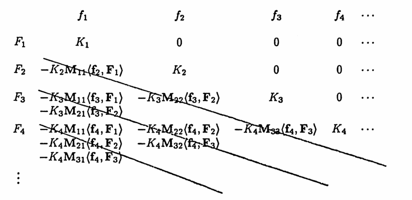
The MATLAB algorithm exploits the following observations regarding the structure of $\,\boldsymbol{\rm M}\,$:
- The numbers $\,K_i\,$ form the main diagonal.
- The element $\,\boldsymbol{\rm M}_{i1}\,$ is easily determined from $\,\boldsymbol{\rm M}_{(i-1),1}\,,$ for $\,i\ge 3\,.$
- Once element $\,\boldsymbol{\rm M}_{i1}\,$ is known, all the entries on the sub-diagonal beginning with $\,\boldsymbol{\rm M}_{i1}\,$ are easily determined.
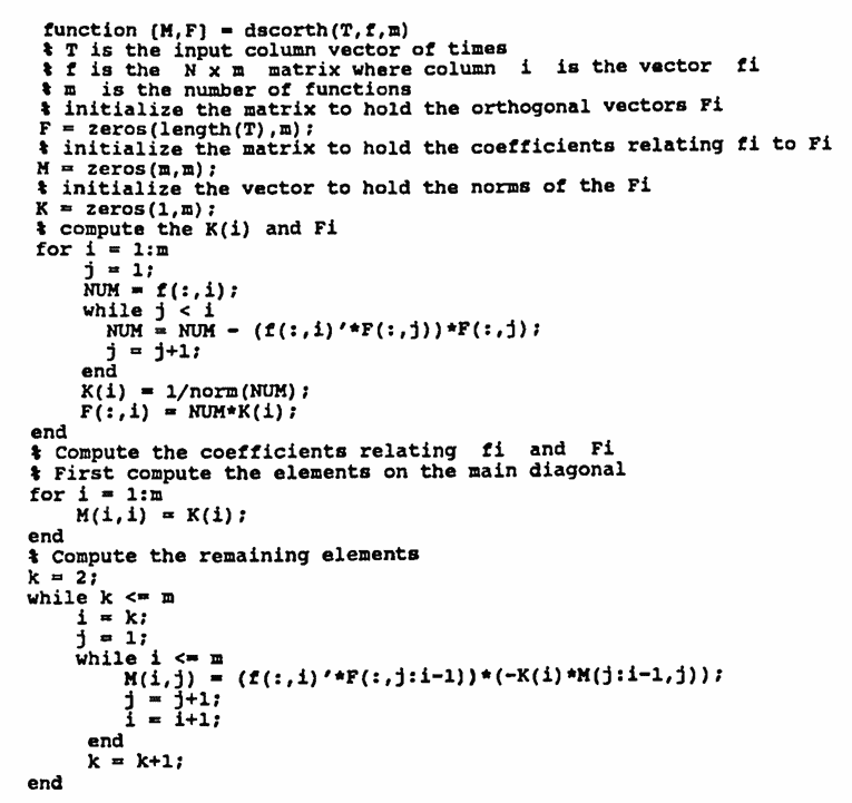
MATLAB IMPLEMENTATION: Converting Functions to Discrete Orthogonal Functions
Let $\,f_1,\ldots,f_m\,$ be $\,m\,$ real-valued functions of a real variable. Let $\,\boldsymbol{\rm T} = (t_1,\ldots,t_N)\,$ be a vector of $\,N\,$ distinct real numbers, where $\,m\le N\,.$
Suppose that the vectors $\,\boldsymbol{\rm f}_i\,,$ defined by
$$ \boldsymbol{\rm f}_i = \bigl( f_i(t_1),\ldots,f_i(t_N) \bigr)\ , $$are linearly independent in $\,\Bbb R^N\,.$
The following MATLAB function produces a matrix $\,\boldsymbol{\rm M}\,$ that contains the coefficients relating the functions $\,f_i\,$ to functions $\,F_i\,$ that are mutually orthogonal with respect to the times values in $\,\boldsymbol{\rm T}\,.$ Precisely, for every $\,i = 1,\ldots,m\,$:
$$ F_i = \boldsymbol{\rm M}_{i1}f_1 + \cdots + \boldsymbol{\rm M}_{im}f_m $$Optionally, the function will return a matrix $\,\boldsymbol{\rm F}\,$ that contains the mutually orthogonal vectors $\,\boldsymbol{\rm F}_i\,,$ with $\,\boldsymbol{\rm F}_i\,$ in column $\,i\,$:
$$ \boldsymbol{\rm F} = \begin{bmatrix} \Rule{0px}{25px}{15px} \,\boldsymbol{\rm F}_1 & | & \boldsymbol{\rm F}_2 & | & \cdots & | & \boldsymbol{\rm F}_m\, \end{bmatrix} $$The matrices $\,\boldsymbol{\rm M}\,$ and $\,\boldsymbol{\rm F}\,$ can then be used to obtain an improved solution to a sensitive least-squares problem
$$ \underset{\boldsymbol{\rm b}\in\Bbb R^m}{\text{min}}\ \|\boldsymbol{\rm y} - \boldsymbol{\rm X}\boldsymbol{\rm b}\|^2\ , $$where $\,\boldsymbol{\rm X}_{ij} = f_j(t_i)\,,$ and where $\,\boldsymbol{\rm X}^t\boldsymbol{\rm X}\,$ has a large condition number, as follows:
-
Replace $\,\boldsymbol{\rm X}\,$ by $\,\boldsymbol{\rm F}\,,$ and use the MATLAB implementation from Section 2.2 to find a vector $\,\boldsymbol{\rm bnew} = (b_1,\ldots, b_m)\,$ so that
$$ f(t) = b_1F_1(t) + \cdots + b_mF_m(t) $$gives the least-squares approximate to the data $\,(t_i,y_i)\,.$
-
Then, use the relationship between the functions $\,f_i\,$ and $\,F_i\,$ (contained in $\,\boldsymbol{\rm M}\,$) to express $\,f(t)\,$ as a linear combination of the original functions $\,f_i\,$:
$$ \begin{align} f(t) &=b_1F_1(t) + \cdots + b_mF_m(t)\cr\cr &= b_1\bigl( \boldsymbol{\rm M}_{11}f_1 + \boldsymbol{\rm M}_{12}f_2 + \cdots + \boldsymbol{\rm M}_{1m}f_m \bigr)\cr &\quad + b_2\bigl( \boldsymbol{\rm M}_{21}f_1 + \boldsymbol{\rm M}_{22}f_2 + \cdots + \boldsymbol{\rm M}_{2m}f_m \bigr)\cr &\quad + \cdots\cr &\quad + b_m\bigl( \boldsymbol{\rm M}_{m1}f_1 + \boldsymbol{\rm M}_{m2}f_2 + \cdots + \boldsymbol{\rm M}_{mm}f_m \bigr)\cr\cr &= f_1\bigl( b_1\boldsymbol{\rm M}_{11} + b_2\boldsymbol{\rm M}_{21} + \cdots + b_m\boldsymbol{\rm M}_{m1} \bigr)\cr &\quad + f_2\bigl( b_1\boldsymbol{\rm M}_{12} + b_2\boldsymbol{\rm M}_{22} + \cdots + b_m\boldsymbol{\rm M}_{m2} \bigr)\cr &\quad + \cdots\cr &\quad + f_m\bigl( b_1\boldsymbol{\rm M}_{1m} + b_2\boldsymbol{\rm M}_{2m} + \cdots + b_m\boldsymbol{\rm M}_{mm} \bigr)\cr\cr\ &:= \tilde b_1f_1(t) + \cdots + \tilde b_m f_m(t) \end{align} $$The coefficients $\,\tilde{\boldsymbol{\rm b}} := (\tilde b_1,\ldots,\tilde b_m)\,$ are obtained by:
$$ \tilde{\boldsymbol{\rm b}} = \boldsymbol{\rm M}^t(\boldsymbol{\rm bnew}) $$
Example
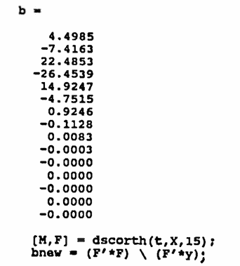
In the following diary of an actual MATLAB session, a data set is fitted with a polynomial of degree $\,14\,,$ in order to illustrate how large condition numbers can cause degraded results, and how the use of discrete orthogonal functions can improve the situation.
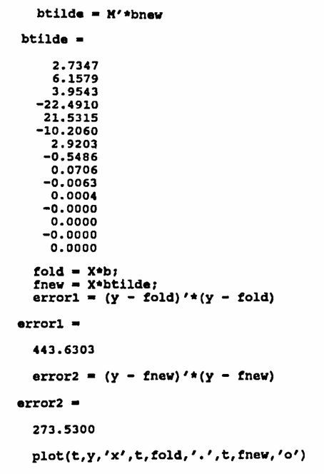
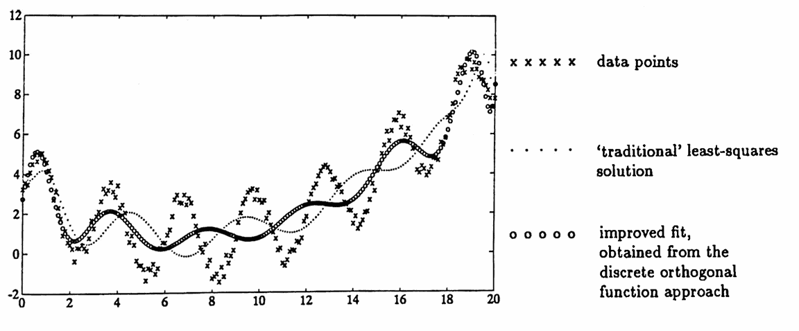
The ‘traditional’ least-squares solution results in a matrix $\,\boldsymbol{\rm X}^t\boldsymbol{\rm X}\,$ with an extremely large condition number, yielding a ‘best fit’ that has error $\,443.6303\,.$
By using the mutually orthogonal function approach, the error is decreased significantly, to $\,273.5300\,.$
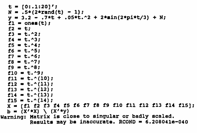
Note: Octave requires two changes:
N = .5*(2*rand(size(t)) - 1);
and
f1 = ones(size(t));