Chapter 2: ‘Fitting’ a Data Set with a Function
2.1 Random Behavior
The Turning Point Test
What is random behavior? For the purposes of this dissertation, a list is called random if the list entries are completely non-deterministic; i.e., if the occurrence of any observation in the list in no way influences the occurrence of any other observation.
Should a list be random, then there is no sense in searching for deterministic components.
This section presents a test for random behavior, called the turning point test. The idea behind the test is this: if data is truly random, then certain behavior dictated by randomness is expected. A probabilistic comparison of properties of the actual data with what is expected—should the data be truly random—is used to support or deny the hypothesis of random behavior.
The turning point test is adapted from [Ken, 21-24]. Several other tests for randomness are discussed in the same cited section.
Some review of probability and statistics concepts is interspersed throughout this section. The reader is referred to [Dghty] for additional material.
A MATLAB program to apply the Turning Point Test is included in this section.
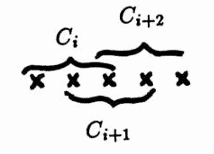
Given an entry $\,y_i\,$ in a list $\,(\ldots,y_{i-1},y_i,y_{i+1},\ldots)\,,$ the adjacent entries $\,y_{i-1}\,$ and $\,y_{i+1}\,$ are called the neighbors of $\,y_i\,.$
An entry in a list is called a peak if it is strictly greater than each neighbor; and is called a trough if it is strictly less than each neighbor.
A list entry is a turning point if it is either a peak or a trough.
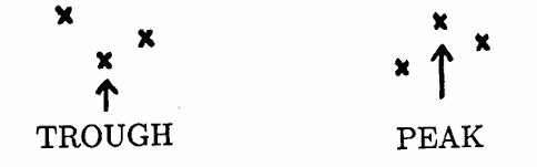
Turning points
The turning point test is so named because it counts the number of turning points in a finite list of data, and compares this number with what is expected, should the data be truly random.
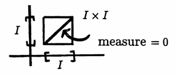
For the turning point test that is developed in this section, it is assumed that the entries in a finite list are allowed to come from an interval of real numbers. Since there are an infinite number of choices for any list entry, the probability that two entries in the list are equal is zero. In particular, the probability that there are equal adjacent entries is zero.
If a finite list contains a large number of duplicate values, then the hypothesis that the list entries come from some interval is probably unwarranted, and the turning point test as developed here will not apply.
$\bigstar\,$ Probability considerations
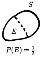
An event $\,E\,$ is a subset of a sample space $\,S\,.$ The probability of $\,E\,$ is determined by how much ‘room’ $\,E\,$ takes up in $\,S\,.$
Suppose that two numbers are chosen from an interval $\,I\,.$ The corresponding sample space is $\,I\times I\,.$ The phrase ‘the probability that there are equal adjacent entries is zero’, means, precisely, that the measure of the set $\{(x,x)\,|\,x\in I\}\,$ (as a subset of $\,I \times I\,$) is zero.
Suppose that three numbers are chosen from an interval $\,I\,.$ The corresponding sample space is $\,I \times I \times I\,.$ The phrase ‘the probability that there are equal adjacent entries is zero’, means, precisely, that the set
$$ S := \{(x,x,y)\,|\,x,y\in I\} \cup \{(x,y,y)\,|\,x,y\in I\}\,, $$(as a subset of $\,I \times I \times I\,$), has measure zero. The set $\,S\,$ is the intersection of two planes in $\,\Bbb R^3\,$ ($\,x = y\,$ and $\,y = z\,$) with the cube $\,I \times I \times I\,$; the resulting set is ‘thin’ in $\,\Bbb R^3\,.$
The hypothesis that the entries in a finite list come from an interval justifies taking the sample space, in the following development of the turning point test, to be all possible arrangements of three distinct values.
If, on the other hand, the entries come from some finite set, then the probability that there are equal adjacent entries is nonzero, and one would have to enlarge the sample space to account for these possible repeat values.
Let $\,\ell\,,$ $\,m\,,$ and $\,g\,$ be three distinct real numbers, with $\,\ell \lt m\lt g\,.$ The letters were chosen to remind the reader of this ordering: $\,\ell\,$ for ‘least’, $\,m\,$ for ‘middle’, and $\,g\,$ for ‘greatest’.
There are $\,3\cdot 2\cdot 1 = 6\,$ ways that these three numbers can be arranged in three slots. If the ordering is random, then these $\,6\,$ possible arrangements will occur with equal probability. Only four arrangements yield a turning point:
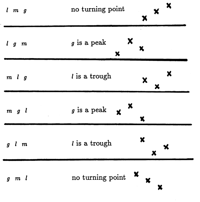
Thus, the probability of finding a turning point in a set of three distinct real values is $\,\frac46 = \frac 23\,.$
Let $\,S\,$ denote the sample space containing all possible arrangements of three distinct values, so that $\,S\,$ contains the six $3$-tuples investigated above.
Define a ‘counting’ random variable $\,C\,:\,S\rightarrow \{0,1\}\,$ via:
$$ C(a,b,c) := \cases{ 1 & \text{if } b \text{ is a turning point}\cr\cr 0 & \text{otherwise}} $$The probability that $\,b\,$ is a turning point is $\,\frac 23\,.$ It follows that the expected value of $\,C\,,$ denoted by both $\,E(C)\,$ and $\,\mu_C\,,$ is:
$$ E(C) = \mu_C = (1)(\frac 23) + (0)(\frac 13) = \frac 23 $$Here, $\,E\,$ is the expected value operator.
Define the function $\,C^2\,$ by:
$$C^2(a,b,c) := C(a,b,c)\cdot C(a,b,c)$$Since $\,1^2 = 1\,$ and $\,0^2 = 0\,,$ it follows that:
$$ C^2(a,b,c) = \cases{ 1 & \text{if}\ b\ \text{ is a turning point}\cr\cr 0 & \text{otherwise}} $$Therefore, $\,E(C^2)\,$ also equals $\,\frac 23\,.$
Let $\,\text{var}(C)\,$ denote the variance of $\,C\,.$ Using the definition of variance, and the linearity of the expected value operator, one computes:
$$ \begin{align} \text{var}(C) &:= E\bigl((C-\mu_C)^2\bigr)\cr &= E(C^2 - 2\mu_CC + \mu_C^2)\cr &= E(C^2) - 2\mu_CE(C) + E(\mu_C^2)\cr &= E(C^2) - 2(\mu_C)^2 + (\mu_C)^2\cr &= E(C^2) - (\mu_C)^2\cr &= \frac 23 - (\frac 23)^2\cr &= \frac 29 \end{align} $$Consider now a list $\,\boldsymbol{\rm y} := (y_1,\ldots,y_n)\,$ of length $\,n\,.$ It is desired to count the number of turning points in this list. Since knowledge of both neighbors is required to classify a turning point, the first and last entries in a list cannot be turning points; so the maximum possible number of turning points present is $\,n - 2\,.$
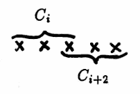
Using the list $\,\boldsymbol{\rm y}\,,$ define $\,C_i\,,$ for $\,i = 2,\ldots,n-1\,,$ by:
$$ C_i(y_{i-1},y_i,y_{i+1}) := \cases{ 1 & \text{if}\ y_i\ \text{is a turning point}\cr\cr 0 & \text{otherwise} } $$Each random variable $\,C_i\,$ is distributed identically to the random variable $\,C\,.$
However, it is important to note that this collection of random variables $\,\{C_i\}_{i=2}^{n-1}\,$ is not a random sample corresponding to $\,C\,,$ because $\,C_i\,$ and $\,C_j\,$ are not independent for $\,0\lt |j-i|\le 2\,$; that is, when the $3$-tuples acted on by $\,C_i\,$ and $\,C_j\,$ overlap. This issue is addressed later on in this section.
Define a random variable $\,T\,$ by:
$$ T := \sum_{i=2}^{n-1} C_i $$Then, $\,T\,$ gives the total number of turning points in the list.
Via linearity of the expected value operator:
$$E(T) = \sum_{i=2}^{n-1} E(C_i) = \frac 23(n-2) := \mu_T $$Next, $\,\text{var}(T)\,,$ the variance of the random variable $\,T\,,$ is computed. Since
$$ \text{var}(T) = E(T^2) - (\mu_T)^2\,, $$one first computes $\,E(T^2)\,$:
$$ \begin{align} E(T^2) &= E\left( \bigl( \sum_{i=2}^{n-1} C_i \bigr)^2 \right)\cr &= E\bigl( (C_2 + \cdots + C_{n-1})^2 \bigr) \end{align} $$There are $ \,(n-2)(n-2) = n^2 - 4n + 4\,$ terms in the product $\,(C_2 + \cdots + C_{n-1})^2\,.$ It is necessary to count the number of terms of the form $\,C_iC_j\,$ for $\,j = i\,,$ $\,|j - i| = 1\,,$ $\,|j - i| = 2\,,$ and $\,|j - i| \gt 2\,$; that is, when the indices on $\,C\,$ are the same, or differ by exactly $\,1\,,$ exactly $\,2\,$, or more than $\,2\,.$
This ‘counting’ is easily accomplished by performing the multiplication as a matrix product, and analyzing the result:
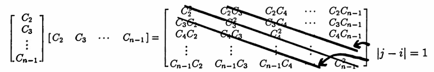
The main diagonal has $\,n-2\,$ entries, each of the form $\,C_i^2\,.$ Thus, there are $\,n-2\,$ terms of the form $\,C_i^2\,.$
There are $\,(n-2)-1 = n-3\,$ entries on the first diagonal above and below the main diagonal, and these are the terms for which $\,|j - i| = 1\,.$ Thus, there are $\,2(n-3)\,$ terms of the form $\,C_iC_{i+1}\,.$
There are $\,(n-2)-2 = n-4\,$ entries on the second diagonal above and below the main diagonal, and these are the terms for which $\,|j-i| = 2\,.$ Thus, there are $\,2(n - 4)\,$ terms of the form $\,C_iC_{i+2}\,.$
The remaining terms are those for which $\,|j - i| \gt 2\,$; thus, there are
$$ \begin{align} &(n^2-4n+4) - (n-2) - 2(n-3)-2(n-4)\cr &\quad = n^2 - 9n + 20\cr &\quad = (n-4)(n-5) \end{align} $$terms of the form $\,C_iC_j\,$ for $\,|j - i| \gt 2\,.$
With a slight abuse of summation notation, the findings thus far are summarized as:
$$ \begin{align} &E(T^2)\cr &\quad = E\left( \bigl( \sum_{i=2}^{n-1} C_i \bigr)^2 \right)\cr &\quad = E\biggl( \sum_{n-2} C_i^2 + \sum_{2(n-3)} C_iC_{i+1} \cr &\qquad \quad + \sum_{2(n-4)} C_iC_{i+2} + \sum_{ \substack{(n-4)(n-5)\\ |j-i|\gt 2}} C_iC_j \biggr) \end{align} \tag{*} $$In each sum, the index denotes the number of terms, and the argument depicts the form of the terms being added. The expectations of each term in (*) must be considered separately.
It has already been observed that $\,E(C_i^2) = \frac 23\,,$ since $\,C_i^2 = C_i\,.$
When $\,|j - i| \gt 2\,,$ the random variables $\,C_i\,$ and $\,C_j\,$ have non-overlapping domains. Under the assumption of randomly generated data, the occurrence or non-occurrence of a turning point for $\,C_i\,$ in no way influences the existence of a turning point for $\,C_j\,$ in this case; i.e., $\,C_i\,$ and $\,C_j\,$ are independent. Thus:
$$ \begin{align} E(C_iC_j) &=E(C_i)\,E(C_j)\cr &=\frac 23\cdot\frac 23 = \frac 49\,,\ \ \text{for}\ |j-i|\gt 2 \end{align} $$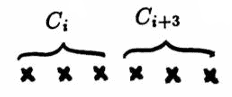
However, for $\,j\le 2\,,$ the random variables $\,C_i\,$ and $\,C_{i+j}\,$ have overlapping domains, and $\,E(C_iC_{i+j}) \ne E(C_i)\,E(C_{i+j})\,$; i.e., $\,C_i\,$ and $\,C_{i+j}\,$ are not independent for $\,j \le 2\,.$
The proof of this statement follows.
To evaluate $\,E(C_iC_{i+1})\,$ requires the investigation of existence of turning points in $\,4\,$ consecutive slots. For convenience of notation, let four distinct real numbers be labeled in order of increasing magnitude as $\,a\,,$ $\,b\,,$ $\,c\,$ and $\,d\,.$ There are $\,4\cdot 3\cdot 2\cdot 1 = 24\,$ ways that these four numbers can be arranged in four slots, as shown below:
| $abcd$ | $bacd$ | $cabd$ | $dabc$ |
| $abdc$ | $badc$ | $cadb$ | $dacb$ |
| $acbd$ | $bcad$ | $cbad$ | $dbac$ |
| $acdb$ | $bcda$ | $cbda$ | $dbca$ |
| $adbc$ | $bdac$ | $cdab$ | $dcab$ |
| $adcb$ | $bdca$ | $cdba$ | $dcba$ |
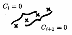
For the arrangement $\,abcd\,,$ $\,C_i = 0\,$ and $\,C_{i+1} = 0\,.$ Thus, $\,C_iC_{i+1} = 0\,.$
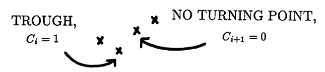
For the arrangement $\,bacd\,,$ $\,C_i = 1\,$ (there is a trough). However, $\,C_{i+1} = 0\,$ (no turning point). Again, $\,C_iC_{i+1} = 0\,.$
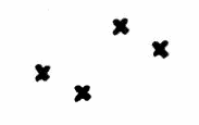
For the arrangement $\,badc\,,$ $\,C_i = 1\,$ (there is a trough), and $\,C_{i+1} = 1\,$ (there is a peak). Thus, $\,C_iC_{i+1} = 1\,.$
Indeed, for the product random variable $\,C_iC_{i+1}\,$ to be nonzero, the arrangement of $\,a\,,$ $\,b\,,$ $\,c\,$ and $\,d\,$ must display both a trough and a peak. This occurs in $\,10\,$ of the $\,24\,$ possible arrangements, and hence:
$$ E(C_iC_{i+1}) = \frac{10}{24} = \frac 5{12} $$Note that $\,\frac{5}{12}\ne \frac 23\cdot\frac 23\,,$ confirming that $\,C_i\,$ and $\,C_{i+1}\,$ are not independent.
The random variables $\,C_i\,$ and $\,C_{i+2}\,$ again have overlapping domains.
To evaluate $\,E(C_iC_{i+2})\,$ requires the investigation of turning points in $\,5\,$ consecutive slots. By methods similar to those just discussed, it can be shown that:
$$ E(C_iC_{i+2}) = \frac{54}{120} = \frac 9{20} $$Substitution of the computed expectations into (*) gives:
$$ \begin{align} &E(T^2)\cr\cr &\quad = \frac 23(n-2) + \frac5{12}\cdot 2(n-3)\cr &\qquad + \frac 9{20}\cdot 2(n-4) + \frac49(n-4)(n-5)\cr\cr &\quad = \cdots = \frac{40n^2 - 144n + 131}{90} \end{align} $$Thus:
$$ \begin{align} \text{var}(T) &= E(T^2) - (\mu_T)^2\cr\cr &= \frac{40n^2 - 144n + 131}{90} - \bigl(\frac23(n-2)\bigr)^2\cr\cr &= \cdots = \frac{16n - 29}{90} \end{align} $$With both the mean and variance of the random variable $\,T\,$ now known, Chebyshev’s Inequality (stated next) can be used to compare the actual number of turning points from a given data set with the number that is expected under the hypothesis of random behavior.
Equivalently:
$$ P\bigl(|X-\mu|\lt t\bigr) \ge 1 - \frac{\sigma^2}{t^2} $$This theorem states that for any random variable $\,X\,$ with mean $\,\mu\,$ and variance $\,\sigma^2\,,$ the probability that $\,X\,$ takes on a value which is at least distance $\,t\,$ from the mean, is at most $\,\frac{\sigma^2}{t^2}\,.$
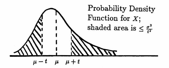
Observe that Chebyshev’s Inequality is a ‘distribution-free’ result; that is, it is independent of the form of the probability density function for $\,X\,.$
It is interesting to note that no ‘tighter’ bound on $\,P(|X - \mu| \ge t)\,$ is possible, without additional information about the actual distribution of $\,X\,.$ That is, there exists a random variable for which equality is obtained in Chebyshev’s Inequality: $\,P(|X - \mu| \ge t) = \frac{\sigma^2}{t^2}\,$ (see, e.g., [Dghty, 123–124]).
Here is how Chebyshev’s Inequality and the turning point test are used to investigate the hypothesis that a given data set is random.
Suppose that a finite list of data values is given, where it is assumed that the entries in the list are allowed to come from some interval of real numbers.
As cautioned earlier, if there are a large number of identical adjacent values in the data set, then the hypothesis that the values come from some interval of real numbers is probably unwarranted, and the turning point test as developed here does not apply.
For any occasional adjacent data values that are identical, delete the repeated value, and decrease $\,n\,$ (the length of the list) by $\,1\,.$ For example, the data list
$$ (1,3,5, \overbrace{2,2},7,6,4,3,9,0,1,5,8) $$of length $\,14\,$ would be transformed to the list
$$ (1,3,5,2,7,6,4,3,9,0,1,5,8) $$of length $\,13\,,$ before applying the turning point test.
Let $\,N\,$ denote the length of the (possibly adjusted) data set.
Let $\,T_{\text{act}}\,$ denote the actual number of turning points in the (adjusted) list. Under the hypothesis of random behavior, the expected value and variance of the random variable $\,T\,$ that counts the number of turning points in the list are given by:
$$ \begin{gather} E(T) = \frac 23(N-2) := \mu\cr\cr \text{and}\cr\cr \text{var}(T) = \frac{16N-29}{90} := \sigma^2 \end{gather} $$Let $\,d := |T_{\text{act}} - \mu|$ denote the distance between the actual and expected number of turning points. By Chebyshev’s Inequality, the probability that the distance of $\,d\,$ or greater between $\,\mu\,$ and $\,T\,$ would be observed, should the data be truly random, is:
$$ P\bigl(|T - \mu|\ge d\bigr) \le \frac{\sigma^2}{d^2} $$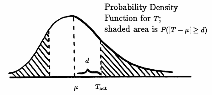
If $\,\frac{\sigma^2}{d^2}\,$ is close to $\,0\,,$ then it is unlikely that $\,T_{\text{act}}\,$ turning points would be observed if the data were truly random. In this case, the hypothesis that the data is random would be rejected, and the search for deterministic components could begin.
If $\,\frac{\sigma^2}{d^2}\,$ is close to $\,1\,,$ then there is no reason to reject the hypothesis of random behavior. In this case, it may be fruitless to search for deterministic components.
Example 1: Applying the Turning Point Test
The data graphed below give the biweekly stock price of a mutual fund over a two-year time period.
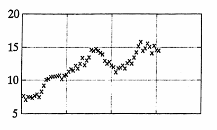
There are no identical adjacent values. The total number of data points is $\,N = 61\,.$
The expected number of turning points, under the hypothesis of random behavior, is:
$$ \mu = \frac 23(N - 2)\approx 39.33 $$The actual number of turning points is
$$ T_{\text{act}} = 28 \,, $$so that the distance between the actual and expected values is:
$$ d := |39.33 - 28| = 11.33 $$The variance of T is:
$$ \begin{align} \sigma^2 &= \frac{16N - 29}{90}\cr\cr &= \frac{16(61)-29}{90}\cr\cr &\approx 10.52 \end{align} $$Chebyshev’s Inequality yields:
$$ P\bigl(|T-\mu|\ge 11.33\bigr) \le \frac{10.52}{(11.33)^2} \approx 0.08 $$Thus, it is quite unlikely that only $\,28\,$ turning points would be observed, if the data were truly random. The hypothesis of random behavior is therefore rejected, and a search for deterministic components can begin.
Some data sets, as in the next example, are ‘locally’ random, and yet exhibit some deterministic behavior from a more ‘global’ point of view. In such instances, short-term data prediction may be unwarranted, whereas longer-term prediction may be possible.
For sufficiently large data sets, the turning point test can be used to help determine the ‘breadth of local random behavior’. This idea is explored in the next example.
Example 2
The data list graphed below was generated within MATLAB by first producing some pure data, via the MATLAB commands
i = [1:100];
y = i/6;
and then introducing noise by use of the MATLAB command rand(A).
The MATLAB command rand(A) produces a matrix the same size as A, with random entries. By default, the random numbers are uniformly distributed in the interval $\,(0,1)\,.$ Then,
2*(rand(A) - 0.5)
gives numbers uniformly distributed in $\,(-1,1)\,.$
The command rand('normal') can be used to switch to a normal distribution with mean $\,0\,$ and variance $\,1\,.$ The command rand('uniform') then switches back to the uniform distribution.
For Octave, the command randn is used to generate random numbers using the standard normal distribution (mean $\,0\,$ and variance $\,1\,$).
Then, the command randn(size(A)) produces a matrix that is the same size as A, with random numbers generated using the standard normal distribution.
The list noisey graphed below was generated by the MATLAB command:
noisey = y + 2*(rand(y) - 0.5);
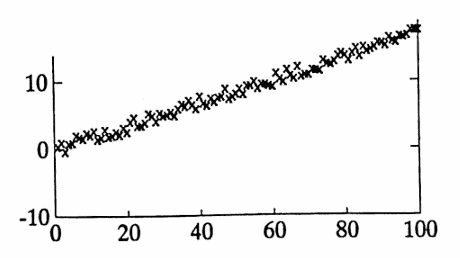
The list noisey has $\,63\,$ turning points, so $\,T_{\text{act}} = 63\,.$
The list noisey has length $\,100\,,$ so $\,N = 100\,,$ and thus $\,\mu = \frac 23(100)\approx 66.67\,$ and $\,\sigma^2 = \frac{16(100)-29}{90} \approx 17.46\,.$
Then, $\,d = |66.67 - 63| = 3.67\,.$
Chebyshev’s Inequality yields:
$$ P\bigl( |T-\mu|\ge 3.67 \bigr) \le \frac{17.46}{(3.67)^2} \approx 1.3 $$Even though the data clearly illustrate a linear ‘trend’, there is no reason, based on this test, to reject the hypothesis of random behavior.
Here is what the turning point test is revealing in this situation: in moving through the list entry-by-entry, the numbers rise and fall in such a way that they could certainly have been produced by an entirely random process.
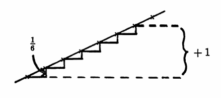
Indeed, since the slope of the ‘pure’ line is $\,\frac 16\,,$ and the noise is $\,\pm 1\,,$ it could take more than $\,6\,$ data entries before any increase due to the linear trend is observed.
Prediction of one data value into the future is unwarranted.
However, if one were to move through the list by taking, say, every fourth entry, then the ‘local’ random behavior may be overshadowed by the ‘global’ linear trend. This idea is investigated in a second, slightly different, application of the turning point test.
Example 2, continued
Generate a new list from noisey, by taking every fourth piece of data. Call the new list noisey4. This is accomplished via the MATLAB command
noisey4 = noisey(1:4:100);
Whereas the time list corresponding to noisey has spacing $\,T = 1\,,$ the time list corresponding to noisey4 has spacing $\,T = 4\,.$ The new list noisey4 is graphed below, and has length $\,N = 25\,.$
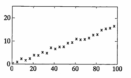
The list noisey4 has $\,10\,$ turning points, so $\,T_{\text{act}} = 10\,.$
The list noisey4 has length $\,25\,,$ so $\,N = 25\,,$ and thus $\mu = \frac 23(25)\approx 16.67\,$ and $\,\sigma^2 = \frac{16(25)-29}{90} \approx 4.12\,.$
Then, $\,d = |16.67 — 10| = 6.67\,.$
Chebyshev’s Inequality yields:
$$ P\bigl(|T-\mu|\ge 6.67\bigr) \le \frac{4.12}{(6.67)^2} \approx 0.09 $$The hypothesis of random behavior is rejected for noisey4. Thus, predicting future values of the list noisey4, based on identified components, may be warranted. In other words, prediction of $\,4\,$ or more days into the future for the original list noisey4 may be warranted.
In this example, the data clearly exhibit a linear trend. A method of ‘fitting’ data with a function of a specific form is discussed in Section 2.2.
In general, it is possible, with sufficient data, to continually produce sublists, xk, of a list x, by taking every $\,k^{\text{th}}\,$ entry from x. If the turning point test, when applied to xk, concludes that the hypothesis of random behavior is rejected, then prediction of $\,k\,$ or more units into the future for the original list x may be warranted.
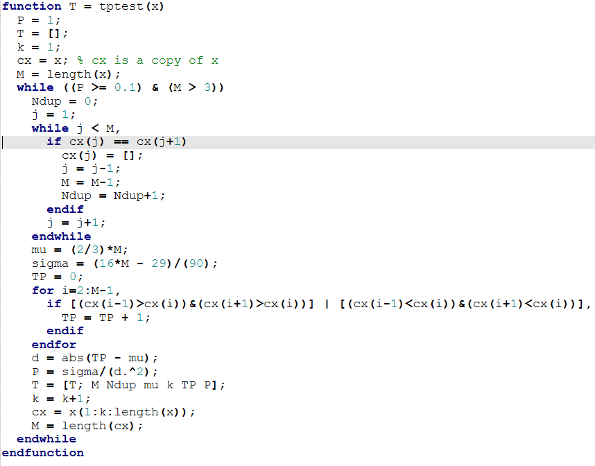
MATLAB FUNCTION: Turning Point Test
The following MATLAB function is used by typing
y = tptest(x)
where: x is the INPUT row or column vector; y is the program OUTPUT.
The output matrix y consists of rows, where each row is of the form:
[length nofdup mu k TP P]
The variable length is the length of the list produced by taking every $\,k^{\text{th}}\,$ entry from x, and adjusting the resulting sublist to account for adjacent identical values. The number of duplicates found in the list is recorded in nofdup.
The variable mu is the expected number of turning points, if the behavior is truly random.
The variable TP is the actual number of turning points.
The variable P is $\,\frac{\sigma^2}{d^2}\,,$ from Chebyshev’s Inequality:
$$ P\bigl( |T-\mu|\ge d \bigr) \le \frac{\sigma^2}{d^2} $$The test is repeatedly applied to sublists, until either the list is depleted, or until P $\lt 0.1\,.$
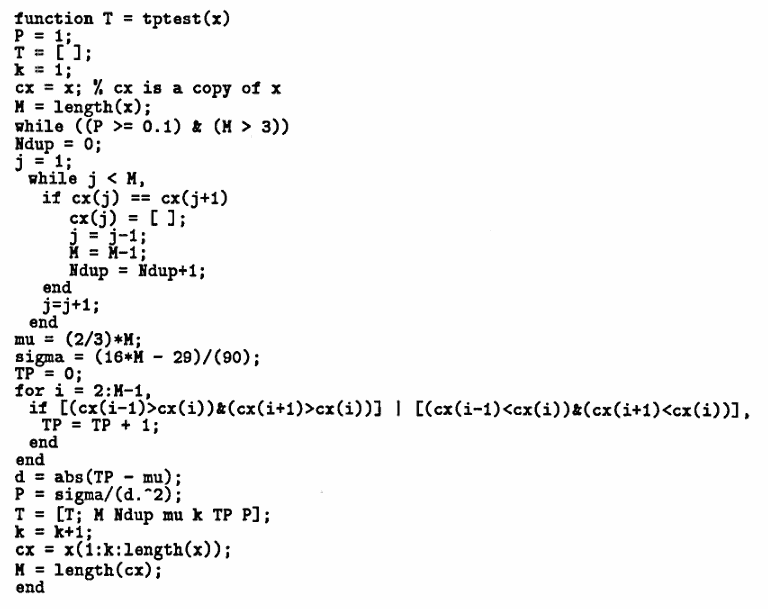
In Octave, the code looks like this:
The following diary of an actual MATLAB session shows the application of this Turning Point Test to the list noisey in Example 2.
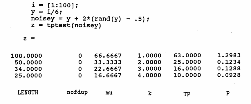
Recall that, in Octave, you must say rand(size(y)) instead of rand(y) .
Economics Application: Taking Advantage of Turning Points
If the hypothesis of random behavior is not rejected for given data, then it may be fruitless to seek deterministic components. However, the economics application discussed in this section shows how one can, even in this situation, often take advantage of the turning points (rises and falls) in stock market data.
The strategy is due to Eliason [Eli]. First, the underlying mathematical theory is presented. Then, an example illustrating the application of this theory to stock market trading is given.
Let $\,\boldsymbol{\rm x}(0)\,$ be a given finite list of real numbers.
Let $\,\boldsymbol{\rm x}(n)\,$ denote the list present at the completion of step $\,n\,$ ($\,n \ge 1\,$) in the Martingale Algorithm (below), where $\,\boldsymbol{\rm x}(0)\,$ is the initial input.
Let $\,A\,:\, \{1,2,3,\ldots\}\rightarrow \{W,L\}\,$ be a given function; for $\,n \ge 1\,,$ either $\,A(n) = W\,$ or $\,A(n) = L\,.$
Let $\,P\,$ and $\,B\,$ be functions,
$$ \begin{gather} P\,:\,\{0,1,2,3,\ldots\}\rightarrow \Bbb R\,,\cr B\,:\,\{0,1,2,3,\ldots\}\rightarrow \Bbb R\,; \end{gather} $$the values assigned to $\,P(n)\,$ and $\,B(n)\,$ (for $\,n \ge 0\,$) are determined by the Martingale Algorithm.
Martingale Algorithm
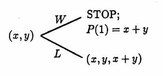
Define $\,P(0) = 0\,.$ If $\,\boldsymbol{\rm x}(0)\,$ has two or more entries, then let $\,B(0)\,$ be the sum of the first and last entries in $\,\boldsymbol{\rm x}(0)\,.$ If $\,\boldsymbol{\rm x}(0)\,$ has only one entry, $\,x\,,$ then let $\,B(0) = x\,.$
If $\,A(n) = W\,,$ then let $\,P(n) = P(n-1) + B(n-1)\,.$ In this case, adjust the list $\,\boldsymbol{\rm x}(n-1)\,$ to get the list $\,\boldsymbol{\rm x}(n)\,,$ as follows:
- If $\,\boldsymbol{\rm x}(n-1)\,$ has more than two entries, then delete the first and last entries to obtain $\,\boldsymbol{\rm x}(n)\,.$
- If $\,\boldsymbol{\rm x}(n-1)\,$ has only one or two entries, then delete these entries, and STOP the algorithm.
If $\,A(n) = L\,,$ then let $\,P(n) = P(n-1) - B(n-1)\,.$ In this case, adjust the list $\,\boldsymbol{\rm x}(n-1)\,$ to get the list $\,\boldsymbol{\rm x}(n)\,,$ by appending $\,B(n-1)\,$ to the end of $\,\boldsymbol{\rm x}(n-1)\,.$
If $\,\boldsymbol{\rm x}(n)\,$ has two or more entries, then let $\,B(n)\,$ be the sum of the first and last entries in $\,\boldsymbol{\rm x}(n)\,.$ If $\,\boldsymbol{\rm x}(n)\,$ has only one entry, $\,x\,,$ then let $\,B(n) = x\,.$ Go to the next value of $\,n\,.$
The variable names used in the Martingale Algorithm are suggestive of common roles that these variables play in applications of the algorithm.
The function $\,A\,$ is the ‘Action’ function; $\,W\,$ denotes a ‘Win’ and $\,L\,$ denotes a ‘Loss’.
The function $\,P\,$ is the ‘Profit’ function, and $\,B\,$ is the ‘Bet’ function. When a WIN occurs, the profit is increased by the previous bet; when a LOSS occurs, the profit is decreased by the previous bet.
Example 1: Applying the Martingale Algorithm
Let $\,\boldsymbol{\rm x} = (1,2,3,5)\,,$ and let $\,A(n) = (L, W, W, L, W,\ldots)\,.$ The table below summarizes the algorithm:
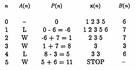
Observe that the algorithm STOPPED at $\,n = 5\,,$ and $\,P(5) = 11 = 1 + 2 + 3 +5\,$; that is, when the algorithm stopped, the value of $\,P\,$ is the sum of the digits in the initial list.
Example 2: Applying the Martingale Algorithm With a Different Action List
Suppose that a different action function is used:
$$ A(n) = (L,L,L,W,L,W,W,\ldots) $$The algorithm is summarized in the table below:
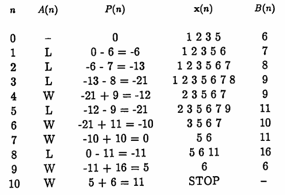
This time, the algorithm stopped at $\,n = 10\,,$ but again $\,P(n) = 11\,.$ The next theorem shows that this behavior is no coincidence:
Let $\,\boldsymbol{\rm x}(0) = (x_1,\ldots,x_m)\,$ be a finite list of real numbers, with $\,m \ge 1\,.$ Let $\,M := x_1 + \cdots + x_m\,$ be the sum of the entries in $\,\boldsymbol{\rm x}(0)\,.$
If a STOP occurs in the Martingale Algorithm at step $\,N\,,$ where $\,\boldsymbol{\rm x}(0)\,$ has been used as the initial input, then $\,P(N) = M\,.$
The number $\,M\,$ is called the series number associated with the list $\,\boldsymbol{\rm x}(0)\,.$
Proof
The proof is by induction.
For $\,n \ge 1\,,$ let $\,T(n)\,$ be the statement:
‘If the algorithm stops at step $\,n\,,$ then $\,P(n) = M\,$’
A series of $\,W\,$’s in the corresponding action list is the quickest way to stop the algorithm. First, action lists containing only $\,W\,$’s are considered. Then, the induction step is applied to action lists that contain at least one $\,L\,.$
If $\,\boldsymbol{\rm x}(0)\,$ has only one entry, $\,\boldsymbol{\rm x}(0) = (x)\,,$ then $\,T(1)\,$ is true (see below).

If $\,\boldsymbol{\rm x}(0)\,$ has two entries, $\,\boldsymbol{\rm x}(0) = (x,y)\,,$ then $\,T(1)\,$ is true (see below).
If $\boldsymbol{\rm x}(0)\,$ has three entries, $\,\boldsymbol{\rm x}(0) = (x, y, z)\,,$ then it takes at least two steps to STOP the algorithm. In this case, $\,T(1)\,$ is vacuously true, and $\,T(2)\,$ is true (see below).
Now suppose $\boldsymbol{\rm x}(0)\,$ has $\,m\,$ entries, $\,\boldsymbol{\rm x}(0) = (x_1,\ldots,x_m)\,,$ where $\,m \ge 4\,.$
If $\,m\,$ is odd, then let $\,m = 2j-1\,$ for $\, j\ge 3\,.$ A series of $\,W\,$’s produces a STOP in $\,j\,$ steps, and $\,T(j)\,$ is true. For $\,1 \le k \lt j\,,$ $\,T(k)\,$ is vacuously true. Only the $\,W\,$’s are shown in the flow chart below.
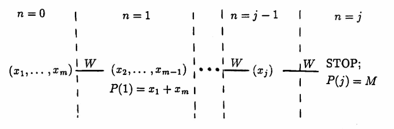
If $\,m\,$ is even, then let $\,m = 2j\,$ for $\,j \ge 2\,.$ A series of $\,W\,$’s produces a STOP in $\,j\,$ steps, and $\,T(j)\,$ is true. For $\,1 \le k \lt j\,,$ $\,T(k)\,$ is vacuously true.
Suppose now that the action list has at least one $\,L\,.$ Suppose that $\,T(k)\,$ is true for all $\,k = 1,\ldots, N - 1\,,$ and consider the statement $\,T(N)\,$.
To motivate what follows, consider a typical flow chart that summarizes all possible actions on a list:
The following observations are important:
- Every STOP at step $\,N\,$ comes from a $\,W\,$ in step $\,N\,.$ Also, in these cases, $\,\boldsymbol{\rm x}(N — 1)\,$ has either $\,1\,$ or $\,2\,$ entries.
- Tracing back from a $\,W\,,$ there is a first $\,L\,,$ say in step $\,N - k\,,$ for $\,1 \le k \le N - 1\,.$
- Taking only $\,W\,$’s from step $\,N - k\,$ leads to a STOP that is earlier than step $\,N\,.$ The inductive hypothesis will be applied to this earlier STOP, to show that $\,T(N)\,$ is true.
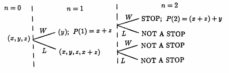
Now, the induction argument. Suppose that a STOP occurs in step $\,N\,,$ and suppose that $\,\boldsymbol{\rm x}(N - 1)\,$ has one entry.
The flow chart below is useful in summarizing the results:
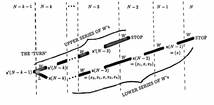
For ease of notation in what follows, the profit functions and lists are denoted by $\,P(n)\,$ and $\,\boldsymbol{\rm x}(n)\,,$ respectively, along the lower series of $\,W\,$’s, and are denoted by $\,P'(n)\,$ and $\,\boldsymbol{\rm x}'(n)\,$ around the TURN and along the upper series of $\,W\,$’s.
- Let $\,\boldsymbol{\rm x}(N - 1) = (x)\,.$ Since $\,P(N) = P(N - 1) + x\,,$ it follows that $\,P(N - 1) = P(N) - x\,.$
- Then, $\,\boldsymbol{\rm x}(N-2) = (x_1,x,x_2)\,$ for real numbers $\,x_1\,$ and $\,x_2\,.$ Since $$ P(N - 1) = P(N - 2) + (x_1 + x_2) \,, $$ it follows that: $$ \begin{align} P(N - 2) &= P(N - 1) - (x_1 + x_2)\cr &= P(N) - (x + x_1 + x_2) \end{align} $$
- Then, $\,\boldsymbol{\rm x}(N - 3) = (x_3,x_1, x, x_2, x_4)\,$ for real numbers $\,x_3\,$ and $\,x_4\,.$ Since $$ P(N - 2) = P(N - 3) + (x_3 + x_4) \,, $$ it follows that: $$ \begin{align} P(N - 3) &= P(N - 2) - (x_3 + x_4)\cr &= P(N) - (x + x_1 + x_2 + x_3 + x_4) \end{align} $$
- Continuing in this fashion, one has, in step $\,N - k\,,$ for $\,2 \le k \le N-1\,$: $$ \begin{align} &\boldsymbol{\rm x}(N — k)\cr &\quad = (x_{2k-3},x_{2k-5},\ldots,x_1,x,x_2,\ldots,x_{2k-4},x_{2k-2})\cr\cr \text{and}\cr\cr &P(N-k)\cr &\quad = P(N) - (x + x_1 + x_2 + \cdots + x_{2k-3} + x_{2k-2}) \end{align} $$
Taking the first $\,L\,$ that occurs in step $\,N — k\,,$ one has:
$$ \boldsymbol{\rm x}'(N - k - 1) = (x_{2k-3},\ldots,x_1,x,x_2,\ldots,x_{2k-4})\,, $$where $\,x_{2k-2}\,$ must equal $\,x_{2k-3}+x_{2k-4}\,,$ since the first and last entries of $\,\boldsymbol{\rm x}'(N-k-1)\,$ are summed and appended to $\,\boldsymbol{\rm x}'(N-k-1)\,$ to produce $\,\boldsymbol{\rm x}(N-k)\,.$
Since
$$ P(N-k) = P'(N-k-1) - (x_{2k-3} + x_{2k-4})\,, $$it follows that:
$$ \begin{align} &P'(N-k-1)\cr\cr &\quad = P(N-k) + (x_{2k-3} + x_{2k-4})\cr &\quad = P(N) - \bigl(x + x_1 + x_2 + \cdots + x_{2k-3} + \overbrace{x_{2k-2}}^{=x_{2k-3}+x_{2k-4}} \bigr)\cr &\qquad + (x_{2k-3} + x_{2k-4})\cr\cr &\quad = P(N) - (x + x_1 + x_2 + \cdots + x_{2k-3}) \end{align} $$Note that $\,\boldsymbol{\rm x}'(N-k-1)\,$ has $\,2k-2 = 2(k-1)\,$ entries. Each successive $\,W\,$ will delete two of these entries, so a STOP will occur in $\,k - 1\,$ steps, that is, in step $\,(N - k - 1) + (k - 1) = N - 2\,.$
Since $\,P'(N-k) = P'(N-k-1) + (x_{2k-3} + x_{2k-4})\,,$ it follows that:
$$ P'(N-k) = P(N)-(x + x_1 + x_2 + \cdots + x_{2k-6} + x_{2k-5}) $$Continuing in this fashion, the remaining $\,k-2\,$ $\,W\,$’s will produce a STOP in step $\,N - 2\,,$ with:
$$ P'(N - 2) = P(N) $$By the inductive hypothesis, $\,P'(N-2) = M\,,$ thus proving that $\,P(N) = M\,.$
In the case where $\,\boldsymbol{\rm x}(N-1)\,$ has two entries, the preceding argument goes through, mutatis mutandis, to show that $\,P'(N-1) = P(N)\,$; and, by the inductive hypothesis, $\,P'(N-1)\,$ equals $\,M\,,$ thus proving that $\,P(N) = M\,.$
Combining results, it has been proven that if a STOP occurs in step $\,N\,,$ then $\,P(N) = M\,,$ thereby showing that $\,T(N)\,$ is true, and completing the proof. $\blacksquare$
Next, the application of this theory to stock market data is given.
Economics Algorithm
Let $\,\boldsymbol{\rm x}(0) = (x_1,\ldots,x_m)\,$ be a list of positive integers to be input into the Martingale Algorithm, with $\,m\gt 1\,.$ Then, the series number $\,M = x_1 + \cdots + x_m\,$ is positive.
Let $\,B\,$ and $\,P\,$ be the functions described in the Martingale Algorithm. Since each list $\,\boldsymbol{\rm x}(n)\,$ in the Martingale Algorithm will have positive entries (since $\,\boldsymbol{\rm x}(0)\,$ does), it follows that $\,B(n)\,$ will be positive, for all $\,n\,.$
Note that $\,B(0) = x_1 + x_m\,,$ and $\,P(0) = 0\,.$
It may be helpful to study Examples $3$ and $4$ as you read through this algorithm.
Let $\,t_0\,$ be some starting time, and let $\,y(t_0)\,$ be the price of a selected stock at time $\,t_0\,.$ In general, $\,y(t)\,$ will denote the price of the stock for $\,t \gt t_0\,.$ The units of $\,y(t)\,$ will typically be dollars.
Let $\,S\,$ (for ‘Shares’) be a positive integer. Shares of stock will be purchased in multiples of $\,S\,.$ Since broker’s fees are usually much smaller when shares are purchased in multiples of $\,100\,,$ $\,S\,$ is typically a multiple of $\,100\,.$
To begin the algorithm, the trader purchases $\,B(0)\cdot S\,$ shares of stock, at price $\,y(t_0)\,.$ The algorithm discussed below will determine future buys and sells of stock.
Let $\,PS\,$ (for ‘Point Spread’) be a fixed positive real number, that will determine when Action (buying or selling of stocks) is to take place, as described next. The units of $\,PS\,$ are the same as the units of $\,y(t)\,.$
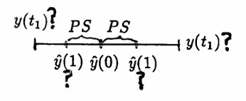
Define $\,\hat y(0) := y(t_0)\,.$ Let $\,t_1 \gt t_0\,$ be a time for which $\,|y(t_1) - \hat y(0)|\ge PS\,$; that is, $\,t_1\,$ is a time at which the price of stock has deviated from the beginning price by $\,PS\,$ or more.
Ideally, (to speed the algorithm to its completion), $\,t_1\,$ will be the first time (after $\,t_0\,$) that the stock price changes by $\,PS\,$ or more.
Define:
$$ \hat y(1) := \cases{ \hat y(0) + PS & \text{if }\ y(t_1) \gt \hat y(0)\cr\cr \hat y(0) - PS & \text{if }\ y(t_1) \lt \hat y(0) } $$Then, $\,\hat y(1)\,$ gives the ‘ideal’ trading price at step $1$; but a broker may not be able to buy/sell at this ‘ideal’ price $\,\hat y(1)\,.$ The value $\,y(t_1)\,$ gives the actual stock price at the time of transaction.
The procedure followed in step $1$ is now repeated for steps $\,2,3,4,\ldots\,.$
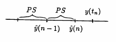
Let $\,t_n \gt t_{n-1}\,$ be a time for which $\,|y(t_n) - \hat y(n-1)| \ge PS\,.$ Define:
$$ \hat y(n) := \cases{ \hat y(n-1) + PS & \text{if }\ y(t_n) \gt \hat y(n-1)\cr\cr \hat y(n-1) - PS & \text{if }\ y(t_n) \lt \hat y(n-1) } $$Then,$\,\hat y(n)\,$ gives the ‘ideal’ trading price at step $\,n\,.$ The value $\,y(t_n)\,$ give the actual stock price at the time of transaction.
For the Economics Algorithm discussed here, it is assumed that the trader is buying long; that is, buying low, with the hopes of selling high. In this case, a rise in stock price is favorable, and is considered to be a WIN; a fall in stock price is unfavorable, and is considered to be a LOSS.
The changes in stock prices (of $\,PS\,$ or more) will determine the ACTION function $\,A\,,$ as follows: a $\,W\,$ (for WIN) is recorded if the stock price increases, and an $\,L\,$ (for LOSS) is recorded otherwise.
For example, suppose that $\,|y(t_n) - \hat y(n-1)| \ge PS\,,$ and $\,y(t_n) \gt \hat y(n-1)\,.$ Then, the price of stock has risen (from the previous ‘ideal’) by $\,PS\,$ or more, and one sets $\,A(n) = W\,.$
If $\,|y(t_n) - \hat y(n-1)| \ge PS\,,$ and $\,y(t_n) \lt \hat y(n-1)\,,$ then the price of stock has fallen (from the previous ‘ideal’) by $\,PS\,$ or more, and one sets $\,A(n) = L\,.$
Define:
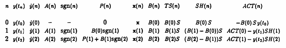
$$ \text{sgn}(n) := \cases{ 1 & \text{if}\ \ A(n) = W\cr -1 &\text{if}\ \ A(n) = L } $$Based on $\,A(n)\,,$ the list $\,\boldsymbol{\rm x}(n-1)\,$ is adjusted, and the number $\,B(n)\,$ is computed, as per the Martingale Algorithm.
The number $\,B(n)\cdot S\,$ gives the number of shares of stock that the trader must own at the completion of step $\,n\,.$ This total number of shares is denoted by $\,TS(n)\,$ in the following table.
In order to own $\,TS(n)\,$ shares, an appropriate number of shares is bought or sold (whichever is appropriate) at price $\,y(t_n)\,.$ The number of shares that must be bought or sold at step $\,n\,$ is denoted by $\,SH(n)\,$ in the following table. If $\,SH(n)\,$ is positive, then shares are purchased; if $\,SH(n)\,$ is negative, then shares are sold.
The account value at the completion of step $\,n\,$ is denoted by $\,ACT(n)\,$ in the following table. If the trader is in debt at the completion of step $\,n\,,$ then $\,ACT(n)\,$ is negative. Otherwise, $\,ACT(n) \ge 0\,.$
Notice that if $\,SH(n)\,$ is positive, then $\,SH(n)\,$ shares are purchased at (positive) price $\,y(t_n)\,,$ and $\,ACT(n) = ACT(n-1) - y(t_n)SH(n)\,.$
On the other hand, if $\,SH(n)\,$ is negative, then $\,-SH(n)\,$ is positive, and $\,-SH(n)\,$ shares are sold at (positive) price $\,y(t_n)\,,$ and $\,ACT(n) = ACT(n - 1) + y(t_n)(-SH(n))\,.$
In both cases:
$$ ACT(n) = ACT(n - 1) - y(t_n)SH(n) $$The algorithm STOPS when the list $\,\boldsymbol{\rm x}(n)\,$ is depleted. At this step, $\,B(n) = 0\,,$ and all shares of stock currently owned are sold.
The table below summarizes the algorithm symbolically. All the symbols used in this table have been discussed in the previous paragraphs.
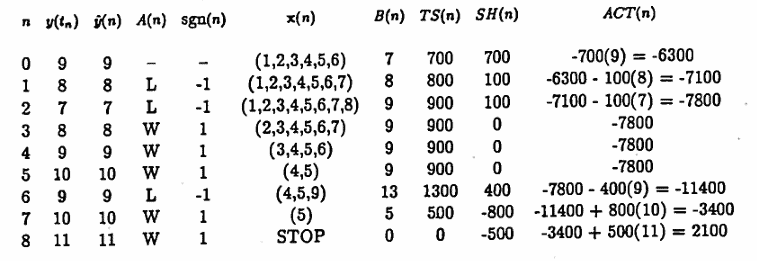
Example 3
The next table illustrates the algorithm in the case where $\,\boldsymbol{\rm x}(0) = (1,2,3,4,5,6)\,,$ the trader is buying long, the rise and fall of stock prices is such that $\,A(n) = (L, L, W, W, W, L, W, W)\,,$ $\,PS = \$1\,,$ $\,S = 100\,,$ and transactions are made at the ‘ideal’ trading prices.
Observe that the series number for $\,\boldsymbol{\rm x}(0)\,$ is $\,21\,,$ and the account value at the completion of the algorithm is:
$$ \$2100 = (PS)\cdot (S)\cdot (\text{series number}) $$The theorem following Example 4 proves that this is no coincidence.
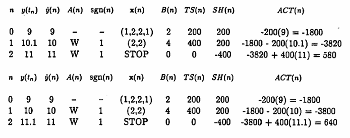
Example 4
The next two tables illustrate that when the actual prices $\,y(t_i)\,$ deviate from the ‘ideal’ prices $\,\hat y(i)\,,$ the end profit may be either higher or lower than the ‘ideal’ profit.
The initial list $\,\boldsymbol{\rm x}(0) = (1,2,2,1)\,$ is used, $\,PS = \$1\,,$ and $\,S = 100\,.$ Thus, the ‘ideal’ profit is $\,\$600\,.$
Let $\,\boldsymbol{\rm x}(0) = (x_1,\ldots,x_m)\,$ be a list of positive integers to be input to the Martingale Algorithm, with $\,m \gt 1\,,$ and with series number $\,M\,.$
Let $\,PS\,$ be a positive real number, and let $\,S\,$ be a positive integer. Let all other notation be as described in the Economics and Martingale Algorithms.
Suppose that all transactions are made at the ideal prices $\,\hat y(n)\,.$
If a STOP occurs in the Economics Algorithm at step $\,N\,,$ then:
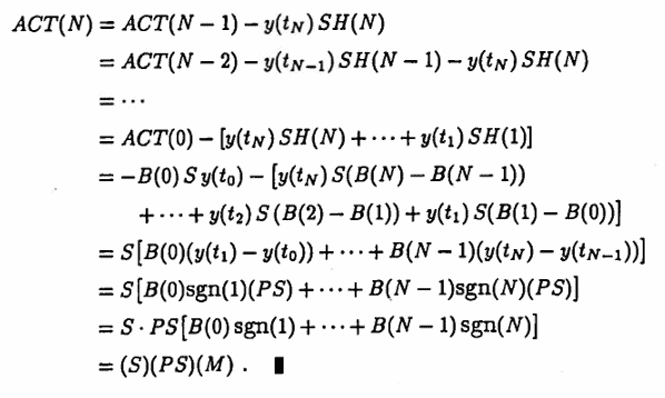
$$ ACT(N) = (S)\cdot(PS)\cdot(M) $$Proof
Suppose that a STOP occurs at step $\,N\,.$ Then, by the Martingale Algorithm Theorem, $\,P(N) = M\,.$ The following expression for $\,P(N)\,$ is obtained:
$$ \begin{align} M &= P(N)\cr &= \strut P(N - 1) + B(N - 1)\text{sgn}(N)\cr &= \strut P(N - 2) + B(N - 2)\text{sgn}(N - 1) + B(N - 1)\text{sgn}(N)\cr &= \strut\cdots\cr &= \strut P(0) + B(0)\text{sgn}(1) + \cdots + B(N - 1)\text{sgn}(N)\cr &= \strut B(0)\text{sgn}(1) + \cdots + B(N - 1)\text{sgn}(N) \end{align} $$Observe also that, under the stated hypotheses:
$$ \begin{align} y(t_i) - y(t_{i-1}) &= \text{sgn}(i)\,|y(t_i) - y(t_{i-1})|\cr &= \strut \text{sgn}(i)(PS) \end{align} $$Observe that:
$$ SH(i) = S\bigl(B(i) - B(i-1)\bigr) $$Now, compute $\,ACT(N)\,$:
The following observations are important:
- Typically, a trader will set two orders with a broker: one action, should a $\,W\,$ occur, and another action, should an $\,L\,$ occur. When the stock price changes by $\,PS\,$ or greater, one order is filled, and the other order is cancelled.
-
The algorithm need not ever STOP. For example, the action list $\,(L,L,L,L,\ldots)\,$ will cause the list $\,\boldsymbol{\rm x}(i)\,$ to continually grow in length.
A MATLAB program for computing the probability that the algorithm STOPS in less than or equal to $\,N\,$ steps is included at the end of this section.
- Even if a STOP does occur, the broker’s fees for transactions may ‘overpower’ the final profit.
- The account value $\,ACT(i)\,$ can get extremely negative, before reaching the final profit.
- Different values of $\,PS\,$ can affect the algorithm dramatically. A proper determination of $\,PS\,,$ based on historical data, is important: many values of $\,PS\,$ should be ‘tested’, and an optimal value chosen.
The reader interested in predictability of stock market prices is referred to [G&M] and [Rosen].
Let $\,N\,$ and $\,m\,$ be positive integers. Suppose that the Martingale Algorithm is started with a list of length $\,m\,.$ Suppose that, at every step, there is equal probability that a $\,W\,$ and $\,L\,$ will occur in the action list; that is:
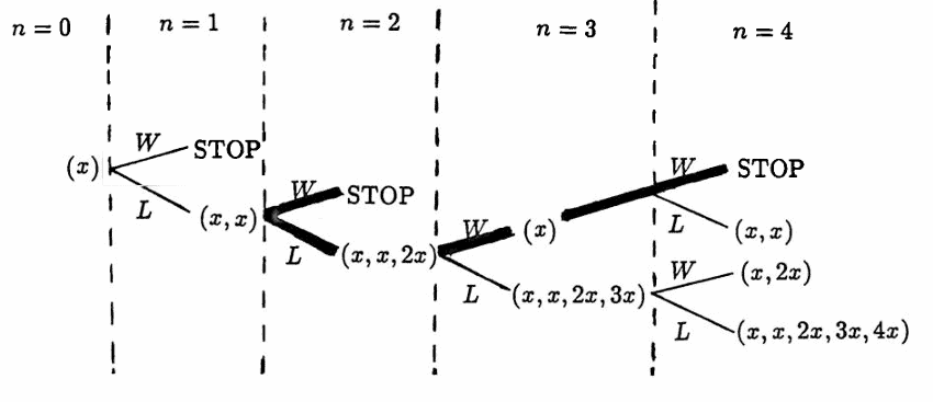
$$ \text{probability}(W) = \text{probability}(L) = 0.5 $$In order to determine the probability that the Martingale Algorithm STOPS in at most $\,N\,$ steps, it is convenient to summarize the flow chart of all possible actions in a diagram such as the one shown below (where $\,m = 1\,$):
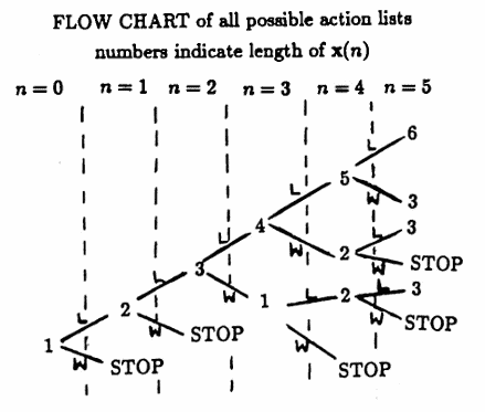
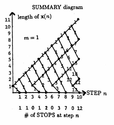
Each point $\,\bigl(n, \text{length of } \boldsymbol{\rm x}(n)\bigr)\,$ in the SUMMARY diagram is called a node.
The numbers on the line segments between nodes in the SUMMARY diagram are called the weights.
Look at the SUMMARY diagram for $\,m = 1\,.$ At step $0\,,$ the list $\,\boldsymbol{\rm x}(0)\,$ has length $\,1\,,$ indicated by the node $\,(0,1)\,.$ A $\,W\,$ in step $1$ results in a STOP, indicated by the node $\,(1,0)\,.$ An $\,L\,$ in step $1$ results in a new list $\,\boldsymbol{\rm x}(1)\,$ of length $2\,,$ indicated by the node $\,(1,2)\,.$
The weights give the number of paths that emanate from the previous node.
For example, consider the node $\,(5,3)\,$ in the SUMMARY diagram. There are two paths in the flow chart that result in a list of length $3$ at step $5$ ending with an $\,L\,$: $\,(L,L,W,L,L)\,$ and $\,(L,L,L,W,L)\,.$ These two paths are indicated by the weight $2$ on the lower line segment leading into the node $\,(5,3)\,.$
There is only one path in the flow chart that results in a list of length $3$ at step $5$ ending with a $\,W\,$: $\,(L, L, L, L, W)\,.$ This path is indicated by the weight $1$ on the upper line segment leading into the node $\,(5,3)\,.$
Observe that each line segment leaving the node $\,(5,3)\,$ has weight $\,2 + 1 = 3\,.$
The nodes of the form $\,(n,0)\,$ correspond to STOPS in the algorithm. The number of STOPS at step $\,n\,$ is summarized along the bottom of the diagram, and is either zero, or equals the weight of the line segment leading into the node.
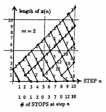
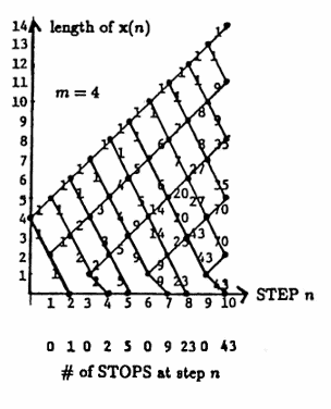
Two more SUMMARY diagrams are given below. The first diagram corresponds to starting length $\,m = 2\,,$ and the second diagram corresponds to starting length $\,m = 4\,.$
The SUMMARY diagrams produced in this manner lend themselves nicely to an algorithm for computing the desired stopping probabilities, as follows.
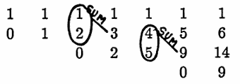
There are ‘upward diagonals’ in each SUMMARY diagram (that is, the lines that have slope $\,1\,$). The weights on each of these diagonals can be associated with a list: the topmost diagonal corresponds to the list $\,(1,1,1,1,1,\ldots)\,$ (for any $\,m\,$). The next diagonal down corresponds to the list $\,(1,2,3,4,5,\ldots)\,$ (for any $\,m\,$).
These lists are arranged in matrix form; every list (except the first) is prefaced with a $\,0\,$ and started in the appropriate column, as illustrated below for the case $\,m = 4\,$:
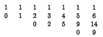
Let $\,M(i,j)\,$ denote the entry (or blank) in row $\,i\,$ and column $\,j\,$ of the arrangement above. For example, $\,M(2,3) = 2\,$ and $\,M(3,6) = 9\,.$ There is no entry in $\,M(3,1)\,.$
The following observations regarding this arrangement of the diagonal lists are important:
- Computation of the probability that the algorithm stops in at most $\,N\,$ steps requires $\,N\,$ columns.
- The starting positions of rows $\,2,3,\ldots\,$ will depend on the starting length $\,m\,.$
-
Once proper starting positions of the rows are computed, the remaining list entries are easily determined as indicated in the example below:
-
The number of STOPS at each step is determined by the lowest (bottom) entry in each column.
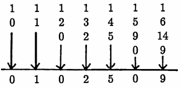
A sample probability is now computed. Let $\,m = 4\,,$ and suppose it is desired to find the probability that the algorithm stops in at most $\,5\,$ steps; denote this by $\,\text{Prob}(N\le 5)\,.$ Let $\,\text{Prob}(N = i)\,$ denote the probability that the algorithm stops in step $\,i\,$ (for $\,i \ge 1\,$). Then:
$$ \begin{align} &\text{Prob}(N\le 5)\cr &\quad = \sum_{i=1}^5 \text{Prob}(N = i)\cr\cr &\quad = \sum_{i=1}^5 ({\small\text{# of STOPS in step $i$})(\text{probability of each STOP}})\cr\cr &\quad = (0)(\frac 12) + (1)(\frac 12)^2 + (0)(\frac 12)^3 + (2)(\frac14)^4 + (5)(\frac12)^5\cr\cr &\quad \approx 0.5313 \end{align} $$Thus, there is a $\,53\%\,$ chance that the algorithm will stop in at most $\,5\,$ steps, when beginning with a list of length $\,4\,.$
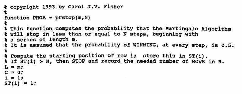
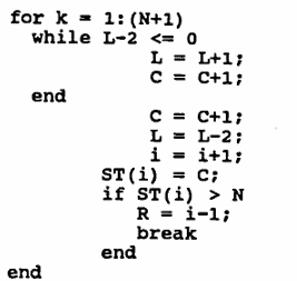
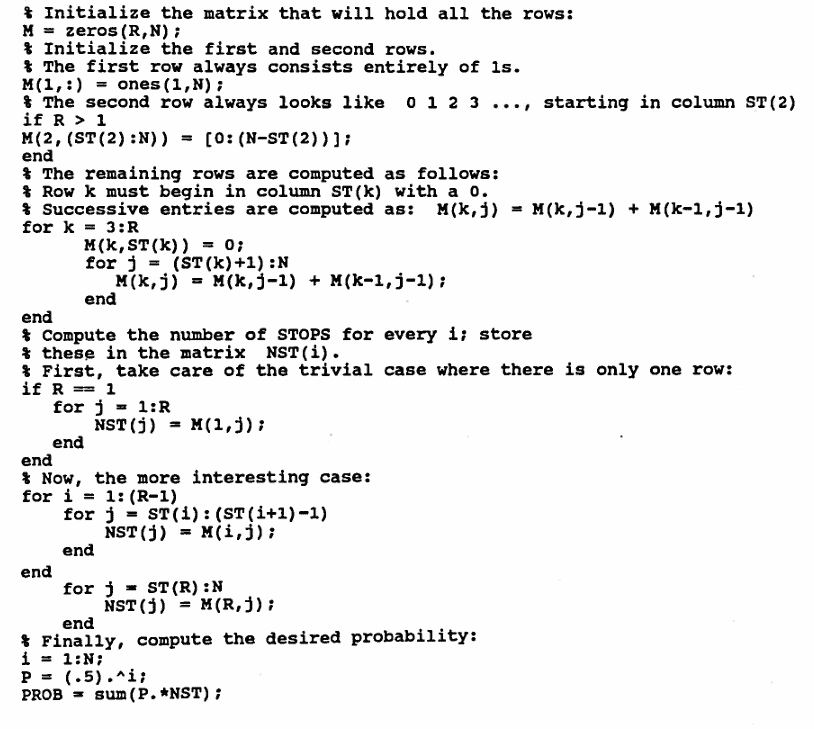
MATLAB Function: prstop(m,N)
The following MATLAB function utilizes the previous observations to compute the desired probabilities.
The reader should store this program in an m-file
named prstop.m.
Then, typing
p = prstop(m,N)from within MATLAB returns a number
p ,
where p is the probability that the
Martingale Algorithm stops in less than or equal to
N steps, starting with a list of length
m , and assuming that, at each step,
$\,\text{Prob}(W) = \text{Prob}(L) = 0.5\,.$
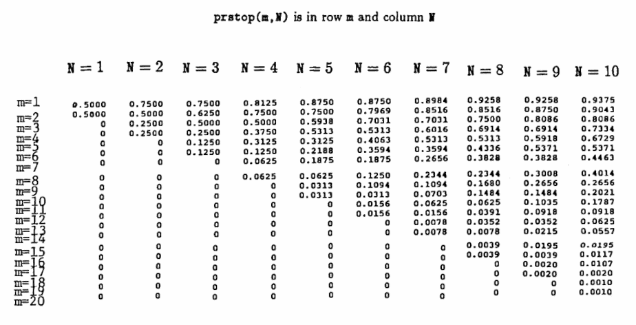
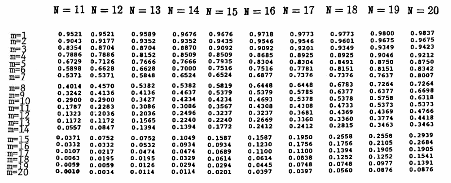
The table following the program lists the probabilities:
prstop(m,N), m = 1,...,20 , N = 1,...,20
The entry in row m
and column N is
prstop(m,M).
endfunction as the final line.
Table:
prstop(m,N) is in row m
and column N