audio read-through Measures of Spread

You may want to review:

Mean and median are measures of central tendency; that is, they each provide a single number that attempts to describe the center of a collection of data.

However, data can be ‘spread out’ around its ‘center’ in very different ways!

This section explores the three most common measures of spread: range, variance, and standard deviation.

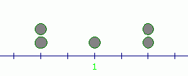
The following data sets all have mean equal to $\,1\,$:

$$ \begin{gather} \cssId{s10}{1,\ \ 1,\ \ 1,\ \ 1,\ \ 1}\cr \cr \cssId{s11}{-1,\ \ 0,\ \ 1,\ \ 2,\ \ 3}\cr \cr \cssId{s12}{-1,\ \ -1,\ \ 1,\ \ 3,\ \ 3} \end{gather} $$

These three data sets are pictured below (as pebbles of equal weight on a number line). Notice that each has its balancing point (mean) at $\,1\,,$ but the data is spread about this mean in very different ways:
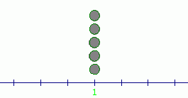
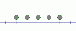
pebbles on a number line: 1,1,1,1,1 pebbles on a number line: -1,0,1,2,3 pebbles on a number line: -1,-1,1,3,3

Clearly, the mean does not capture any information about the spread or variability of data about the mean.

First, we discuss the simplest measure of spread—the range.

DEFINITION range

Let $\ x_{\text{max}}\ $ and $\ x_{\text{min}}\ $ denote the greatest and least numbers in a (finite) data set, respectively.

The range of the data set is the difference: $$ \cssId{s23}{ x_{\text{max}} - x_{\text{min}}} $$

Thus, the range is the difference between the greatest and least numbers in the data set. Since $\, x_{\text{max}}\, $ is always greater than or equal to $\, x_{\text{min}}\,,$ it follows that the range is always greater than or equal to zero.

Examples

The range of the data set  $\ 1,\ 1,\ 1,\ 1,\ 1\ $   is  $\,1 - 1 = 0\,.$
The range of the data set  $\ -1,\ 0,\ 1,\ 2,\ 3\ $   is  $\,3 - (-1) = 4\,.$
The range of the data set  $\ -1,\ -1,\ 1,\ 3,\ 3\ $   is also  $\,3 - (-1) = 4\,.$

Since computation of the range uses only two members from a data set, it is necessarily incomplete in the information that it provides. However, the range is extremely easy to compute.

Another reasonable way to measure the spread takes into account how far each data element is from the mean:

DEFINITION deviation from the mean

Suppose a data set has mean $\,\bar{x}\,,$ and let $\,x_i\,$ denote an element in this data set.

The deviation of $\,x_i\,$ from the mean is given by the formula:

$$ \cssId{s44}{x_i - \bar{x}} $$

From this definition, it is apparent that:

Merely summing the deviations from the mean is useless as a measure of spread because the sum of all the deviations is always equal to zero, as the following calculation shows:

$$ \begin{align} &\cssId{s52}{\sum_{i=1}^n\ (x_i - \bar{x})}\cr\cr &\quad\cssId{s53}{=\ (x_1 - \bar{x}) + (x_2 - \bar{x}) + \cdots + (x_n - \bar{x})}\cr\cr &\quad\cssId{s54}{=\ (x_1 + x_2 + \cdots + x_n) - n\bar{x}}\cr\cr &\quad\cssId{s55}{=\ n\cdot \frac{x_1 + x_2 + \cdots + x_n}{n} - n\bar{x}}\cr &\qquad\cssId{s56}{(\text{multiply first part by 1})}\cr\cr &\quad\cssId{s57}{=\ n\bar{x} - n\bar{x}}\cr\cr &\quad\cssId{s58}{=\ 0} \end{align} $$

Read-Through, Part 2

Also, we don't usually care whether data elements lie above or below the mean; we're more interested simply in the distances from the mean.

A reasonable idea is to sum the absolute values of the deviations from the mean, $\,|x_i - \bar{x}|\,.$ However, the absolute value function is not particularly easy to work with mathematically.

Instead, we get a good measure of spread by summing the squares of the deviations from the mean, $\,(x_i -\bar{x})^2\,.$ There's just one little problem to resolve first.

DEFINITIONS population, sample
The entire collection of individuals or objects about which information is desired is called the population.

A nonempty proper subset (choosing some, but not all) of the population is called a sample.

The formulas for the population mean and the sample mean are identical: add up the numbers, and divide by how many there are.

The population mean is denoted by $\,\mu\,$ and a sample mean is denoted by $\,\bar{x}\,.$ In general, population statistics are reported using Greek letters, like $\,\mu\,$ (mu) and $\,\sigma\,$ (sigma). However, sample statistics are reported using Roman letters, like $\,x\,$ and $\,s\,.$

The common formulas for measures of spread are slightly different, depending upon whether you're looking at the entire population, or just a sample from this population, as shown next:

DEFINITIONS population variance, population standard deviation

Suppose a population has $\,N\,$ data values with mean $\,\mu\,.$

The variance of the population, denoted by $\,\sigma^2\,,$ is given by the formula $$ \cssId{sb35}{\sigma^2 = \frac{\sum\ (x-\mu)^2}{N}}\ , $$ where the sum is over all data values $\,x\,$ in the population.

The standard deviation of the population, denoted by $\,\sigma\,,$ is the square root of the variance: $$ \cssId{sb40}{\sigma = \sqrt{\sigma^2} = \sqrt{\frac{\sum\ (x-\mu)^2}{N}}} $$

Thus, to find the variance of a population, you sum the squared deviations from the mean, and then divide by the number of data values.

DEFINITIONS sample variance, sample standard deviation

Suppose a sample has $\,n\,$ data values with sample mean $\,\bar{x}\,.$

The sample variance, denoted by $\,s^2\,,$ is given by the formula $$ \cssId{sb51}{s^2 = \frac{\sum\ (x-\bar{x})^2}{n-1}}\ , $$ where the sum is over all data values $\,x\,$ in the sample.

The sample standard deviation, denoted by $\,s\,,$ is the square root of the sample variance: $$ \cssId{sb56}{s} \cssId{sb57}{= \sqrt{s^2}} \cssId{sb58}{= \sqrt{\frac{\sum\ (x-\bar{x})^2}{n-1}}} $$

Observe the difference between population variance and sample variance: for the sample variance, you divide by one less than the number of data values , instead of the actual number of data values. Why is this?

Here's one way to understand why: if you randomly choose a sample from a population, what's the likelihood that you'll choose both the greatest and the least values, to represent the true variability in the data set? Not much!

A sample tends to underestimate the true variability in a population.

To compensate, we divide by $\,n-1\,$ instead of $\,n\,$; dividing by a smaller number adjusts the result so it's a bit larger. (The precise reason that you divide by $\,n-1\,$ is explored in a college-level statistics course.)

Standard deviation has a couple advantages over variance:

To conclude, let's return to the three simple data sets presented at the start of this lesson, and compute their measures of spread.

When computing sample variance and sample standard deviation, assume that the given data is part of some (unknown) larger population.

Examples

Question:  Consider the data set $\,\{1,1,1,1,1\}\,.$ $$ \begin{gather} \cssId{sb82}{\text{mean }} \cssId{sb83}{= \frac{1+1+1+1+1}5} \cssId{sb84}{= \color{red}{1}}\cr\cr \cssId{sb85}{\text{range }} \cssId{sb86}{= 1 - 1} \cssId{sb87}{= 0}\cr\cr \end{gather} $$ $$ \begin{align} &\cssId{sb88}{\text{population variance }} \cr &\quad \cssId{sb89}{= \sigma^2} \cr &\quad \cssId{sb90}{= {\textstyle\frac{(1-\color{red}{1})^2 + (1-\color{red}{1})^2 + (1-\color{red}{1})^2 + (1-\color{red}{1})^2 + (1-\color{red}{1})^2}5}}\cr &\quad \cssId{sb91}{= 0}\cr\cr &\cssId{sb92}{\text{population standard deviation }} \cr &\quad \cssId{sb93}{= \sigma}\cr &\quad \cssId{sb94}{= \sqrt{0}}\cr &\quad \cssId{sb95}{= 0}\cr\cr \end{align} $$ $$ \begin{align} &\cssId{sb96}{\text{sample variance }}\cr &\quad \cssId{sb97}{= s^2}\cr &\quad \cssId{sb98}{= {\textstyle\frac{(1-\color{red}{1})^2 + (1-\color{red}{1})^2 + (1-\color{red}{1})^2 + (1-\color{red}{1})^2 + (1-\color{red}{1})^2}4}}\cr &\quad \cssId{sb99}{= 0}\cr\cr &\cssId{sb100}{\text{sample standard deviation }}\cr &\quad \cssId{sb101}{= s}\cr &\quad \cssId{sb102}{= \sqrt{0}}\cr &\quad \cssId{sb103}{= 0} \end{align} $$

Notice that the variance, standard deviation, and range all reflect the fact that there is absolutely no variability about the mean in this data set.

Question:  Consider the data set $\,\{-1,0,1,2,3\}\,.$ $$ \begin{gather} \cssId{sb107}{\text{mean }} \cssId{sb108}{= \frac{-1+0+1+2+3}5} \cssId{sb109}{= \frac{5}{5}} \cssId{sb110}{= \color{red}{1}}\cr\cr \cssId{sb111}{\text{range }} \cssId{sb112}{= 3 - (-1)} \cssId{sb113}{= 4}\cr\cr \end{gather} $$ $$ \begin{align} &\cssId{sb114}{\text{population variance }}\cr &\quad \cssId{sb115}{= \sigma^2}\cr &\quad \cssId{sb116}{= {\textstyle\frac{(-1-\color{red}{1})^2 + (0-\color{red}{1})^2 + (1-\color{red}{1})^2 + (2-\color{red}{1})^2 + (3-\color{red}{1})^2}5}}\cr &\quad \cssId{sb117}{= \frac{10}{5}}\cr &\quad \cssId{sb118}{= 2}\cr\cr &\cssId{sb119}{\text{population standard deviation }} \cr &\quad \cssId{sb120}{= \sigma}\cr &\quad \cssId{sb121}{= \sqrt{2}}\cr &\quad \cssId{sb122}{\approx 1.4}\cr\cr \end{align} $$ $$ \begin{align} &\cssId{sb123}{\text{sample variance }}\cr &\quad \cssId{sb124}{= s^2}\cr &\quad \cssId{sb125}{= {\textstyle\frac{(-1-\color{red}{1})^2 + (0-\color{red}{1})^2 + (1-\color{red}{1})^2 + (2-\color{red}{1})^2 + (3-\color{red}{1})^2}4}}\cr &\quad \cssId{sb126}{= \frac{10}{4}}\cr &\quad \cssId{sb127}{= 2.5}\cr\cr &\cssId{sb128}{\text{sample standard deviation }}\cr &\quad \cssId{sb129}{= s}\cr &\quad \cssId{sb130}{= \sqrt{2.5}}\cr &\quad \cssId{sb131}{\approx 1.6} \end{align} $$
Question:  Consider the data set $\,\{-1,-1,1,3,3\}\,.$ $$ \begin{gather} \cssId{sb134}{\text{mean }} \cssId{sb135}{= \frac{-1+(-1)+1+3+3}5} \cssId{sb136}{= \frac{5}{5}} \cssId{sb137}{= \color{red}{1}}\cr\cr \cssId{sb138}{\text{range }} \cssId{sb139}{= 3 - (-1)} \cssId{sb140}{= 4}\cr\cr \end{gather} $$ $$ \begin{align} &\cssId{sb141}{\text{population variance }}\cr &\quad \cssId{sb142}{= \sigma^2}\cr &\quad \cssId{sb143}{= {\textstyle\frac{(-1-\color{red}{1})^2 + (-1-\color{red}{1})^2 + (1-\color{red}{1})^2 + (3-\color{red}{1})^2 + (3-\color{red}{1})^2}5}}\cr &\quad \cssId{sb144}{= \frac{16}{5}}\cr &\quad \cssId{sb145}{= 3.2}\cr\cr &\cssId{sb146}{\text{population standard deviation }}\cr &\quad \cssId{sb147}{= \sigma}\cr &\quad \cssId{sb148}{= \sqrt{3.2}}\cr &\quad \cssId{sb149}{\approx 1.8}\cr\cr \end{align} $$ $$ \begin{align} &\cssId{sb150}{\text{sample variance }} \cr &\quad \cssId{sb151}{= s^2}\cr &\quad \cssId{sb152}{= {\textstyle\frac{(-1-\color{red}{1})^2 + (-1-\color{red}{1})^2 + (1-\color{red}{1})^2 + (3-\color{red}{1})^2 + (3-\color{red}{1})^2}4}} \cr &\quad \cssId{sb153}{= \frac{16}{4}}\cr &\quad \cssId{sb154}{= 4}\cr\cr &\cssId{sb155}{\text{sample standard deviation }}\cr &\quad \cssId{sb156}{= s} \cr &\quad \cssId{sb157}{= \sqrt{4}}\cr &\quad \cssId{sb158}{= 2} \end{align} $$

Jump up to wolframalpha.com and type in, say:

{-1,-1,1,3,3}

Voila! Instant statistics! How easy is that?

Concept Practice