2.5 Cubic Spine Interpolation

Occasionally, an analyst may choose to ‘fill in’ (interpolate) some missing values in a data set—perhaps to achieve a uniform time list, or to replace a data point that is clearly in error.

The validity of such replacement of actual data with artificial data should always be carefully considered. When it is decided that such a replacement should take place, then splines are a useful tool for determining the replacement data value(s).

In mathematical literature, a spline is a function formed by piecing together other functions, achieving some degree of smoothness (differentiability) in the final ‘pieced together’ curve.

Splines have applications in graphics, where, for example, a set of points must be connected with a smooth curve or surface [Prenter, Chap. 5]. Splines also have applications in the numerical solutions of partial and differential equations [Prenter, Chaps. 7&8].

The current section discusses an important class of spline functions, called cubic splines, and MATLAB implementation of the ideas herein.

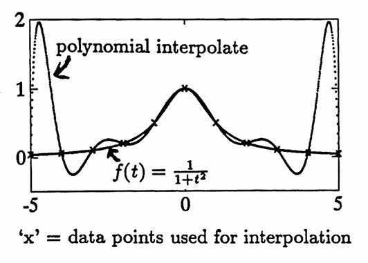
When polynomials are used to interpolate data, it is possible to get large oscillations between data points.

This phenomenon is illustrated in the graph below, where a polynomial is fitted to uniformly-spaced data points from the function $\,f(t) = \frac 1{1 + t^2}\,.$

Splines offer an interpolation approach that does not yield such oscillations.

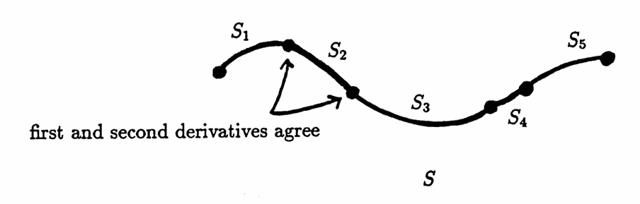
Roughly, a cubic spline is a function formed by patching together cubic polynomials, forcing the function values, first and second derivatives to agree at the patching points. In this way, a curve is obtained that has a continuous second derivative.

The cubic polynomial on the $\,i^{\text{th}}\,$ subinterval is called $\,S_i\,.$ The entire spline (formed from the pieced-together cubics) is called $\,S\,.$

The ideas behind cubic spline interpolation can be illustrated using just three data points; call them:

These points need not be equally spaced. In the context of splines, interpolating points are commonly referred to as ‘knots’ .

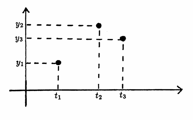
The $t$-values of these three data points naturally yield two subintervals, $\,[t_1, t_2]\,$ and $\,[t_2, t_3]\,,$ called the first and second subinterval, respectively.

On the first subinterval, let:

Similarly, on the second subinterval, let:

The following naming convention is used for the polynomial coefficients:

• The first subscript in the coefficient $\,c_{ij}\,$ agrees with the subscript on $\,S_i\,,$ and gives the subinterval on which $\,S_i\,$ is defined. Thus, $\,S_1\,$ is a cubic polynomial on the first subinterval, which has coefficients $\,c_{1j}\,.$
• The second subscript in the coefficient $\,c_{ij}\,$ tells the power of $\,t\,$ that the coefficient multiplies. For example, $\,c_{10}\,$ multiplies the $\,t^0\,$ (constant) term, and $\,c_{13}\,$ multiplies the $\,t^3\,$ term.

The cubic spline is formed by appropriately patching together $\,S_1\,$ and $\,S_2\,.$ Observe that there are $\,8\,$ unknown coefficients: $\,c_{10},\ldots,c_{13},c_{20},\ldots,c_{23}\,.$ Thus, due to the linear nature of the problem, $\,8\,$ pieces of (non-overlapping, non-contradictory) information are needed to solve uniquely for these coefficients.

Requiring that the curves pass through the appropriate data points yields $\,4\,$ equations:

Requiring that the first and second derivatives agree at the ‘patching point’ yields $\,2\,$ more equations:

There are two additional pieces of information needed.

Observe that the resulting spline function $\,S\,$ will only be defined on the interval $\,[t_1,t_3]\,.$ Therefore, $\,S\,$ is useless for predictive purposes.

Here is the scenario when there are $\,N \ge 2\,$ data points: in this case, there are $\,N-1\,$ subintervals, and hence $\,N-1\,$ cubic polynomials being patched together. Thus, there are $\,4(N-1) = 4N-4\,$ unknowns.

Requiring that the spline pass through the data points yields $\,2\,$ equations (for the endpoints), plus $\,2(N-2)\,$ equations (for the interior points). This gives a total of $\,2 + 2(N-2) = 2N-2\,$ equations.

Requiring that the first and second derivatives agree at the interior points yields another $\,2(N-2) = 2N - 4\,$ equations.

Together, this yields $\,(2N-2) + (2N-4) = 4N-6\,$ equations. Again, two additional equations are required to reach the number of unknowns, $\,4N - 4\,.$

One way to impose the remaining two conditions is to require that the second derivative be zero at the endpoints; for the situation where there are only three points, this gives:

The resulting spline is called the ‘natural’ cubic spline function. A program for computing natural cubic splines is included at the end of this section.

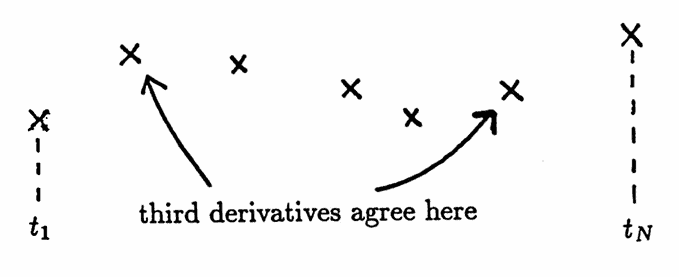
There are other ways to impose the remaining two conditions. For example, the ‘not-a-knot’ condition requires that:

In this case, the functions $\,S_1\,$ and $\,S_2\,$ agree in function value, first, second and third derivatives at $\,t_2\,,$ from which it follows that $\,S_1\,$ is identical to $\,S_2\,.$

Similarly, the functions $\,S_{N-2}\,$ and $\,S_{N-1}\,$ must be identical. Hence, the points $\,(t_2,y_2)\,$ and $\,(t_{N-1},y_{N-1})\,$ are not knots, and the name is appropriate.

The built-in MATLAB  spline  command uses the ‘not-a-knot’ condition.

The natural cubic spline has the property that it minimizes the integral

over all possible functions $\,f\,$ that have continuous second derivatives on the interval $\,[t_1, t_3]\,$ [S&B, p. 96]. What is the significance of this minimization property? The answer lies in the fact that the second derivative of a function measures how ‘curvy’ that function is, as follows:

Recall that if a function $\,f\,$ is differentiable at $\,t\,,$ then $\,f'(t)\,$ gives the instantaneous rate of change of the function values $\,f(t)\,$ with respect to the inputs $\,t\,,$ at the point $\,(t,f(t))\,.$

If $\,f\,$ is twice differentiable at $\,t\,,$ then the second derivative $\,(f')'(t) := f''(t)\,$ gives the instantaneous rate of change of the slopes $\,f'(t)\,$ with respect to $\,t\,$; that is, $\,f''\,$ measures how fast the curve ‘turns’ .

For example, if the second derivative is large and positive, then the slopes increase quickly; and if the second derivative is small and positive, the slopes increase slowly:

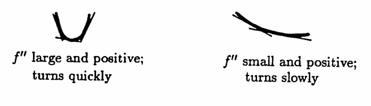
In this way, the second derivative is a measure of ‘curviness’ . The integral $\,\int_{t_1}^{t_3} \bigl(f''(t)\bigr)^2\,dt\,$ ‘sums’ the contributions of $\,\bigl(f''(t)\bigr)^2\,$ on the interval $\,[t_1,t_3]\,.$ (The quantity $\,f''(t)\,$ is squared, since one is only interested in the magnitude of $\,f''\,,$ and not its sign.)

Thus, the number $\,\int_{t_1}^{t_3} \bigl(f''(t)\bigr)^2\,dt\,$ is a measure of the ‘curviness’ of the function $\,f\,$ on the interval $\,[t_1,t_3]\,.$ With respect to this measure of ‘curviness’ , the natural cubic spline is the least curvy interpolate of the data points, over all possible interpolates that have a continuous second derivative.

In practice, the natural cubic spline is very similar to the ‘not-a-knot’ spline. One example, illustrating how closely they agree, is included at the end of this section.

Returning to the simple case of three data points, the $\,8\,$ imposed conditions for the natural cubic spline can be rewritten in terms of the coefficients $\,c_{ij}\,,$ yielding a system of $\,8\,$ equations in $\,8\,$ unknowns.

Observe that with

one has

and:

The $\,8\,$ constraints for the natural cubic spline are therefore

or, in matrix form:

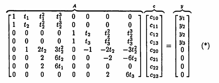
For convenience, denote this in the form $\,Ac = y\,,$ with appropriate definitions for $\,A\,,$ $\,c\,$ and $\,y\,.$ It can be shown that the matrix $\,A\,$ is always invertible [S&B, p. 101], so the coefficients are given (at least theoretically) by:

Example

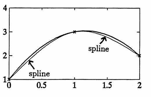
As a simple example, the natural cubic spline through the three data points

is computed. The matrix (*) becomes:

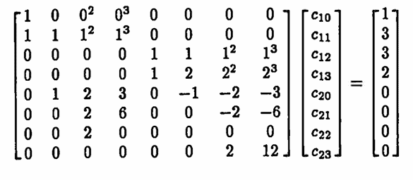
Solution of this system (here, using MATLAB) yields the $\,c\,$ column vector:

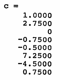
The spline is graphed below. On the same graph is shown the unique parabola (degree $\,2\,$ polynomial) that passes through these three points. Observe that the spline is ‘less curvy’ than the parabola. (To see this, note that the ‘least curvy’ path between, say, the points $\,(0,1)\,$ and $\,(1,3)\,,$ is the line segment connecting these two points—and the spline is closer to this line segment.)

One has probably noted that the matrix $\,A\,$ in the system (*) gets very large, very fast, as the number of data points increases. Numerical methods to compute splines take a dramatically different approach to the problem, which results in smaller matrix sizes. The interested reader is referred to [S&B, 97–102] for details.

MATLAB IMPLEMENTATION: Polynomial and Spline Interpolation

MATLAB provides built-in commands for polynomial approximation and interpolation, and for cubic spline interpolation (with the ‘not-a-knot’ condition).

In what follows, let  t  be a vector containing the time values of a data set $\,\{(t_i,y_i)\}_{i=1}^N\,,$ and let  y  be a vector containing the corresponding data values. The entries of  t  should all be distinct. There are $\,N\,$ data points.

The command

p = polyfit(t,y,k)

fits the data set with a polynomial of degree $\,k\,.$ The returned vector  p  contains the coefficients of the fitting polynomial, $\,p(t)\,,$ in descending powers of $\,t\,.$

If $\,k \ge N-1\,,$ then the resulting polynomial will pass through all the data points; in this case, the polynomial is an interpolate of the data set. If $\,k \lt N - 1\,,$ then the resulting polynomial fits the data in a least-squares sense.

The output  p  from the previous command can be input into the  polyval  (‘polynomial values’) command, in order to plot the ‘fitting’ polynomial. Whenever  p  is a vector whose elements are the coefficients of a polynomial in descending powers, then the command

 yfit = polyval(p,tfine)

returns a vector  yfit  that contains the polynomial  p  evaluated at each element in  tfine . The command

 plot(tfine,yfit,'.')

can then be used to view the fitting polynomial.

Let $\,S\,$ be the ‘not-a-knot’ cubic spline that passes through the data points $\,\{(t_i,y_i)\}_{i=1}^N\,.$ Let  t  and  y  be vectors containing the time and data values, respectively, and let  tfine  be a vector containing numbers from the interval $\,[t_1,t_N]\,.$ The command

yspl = spline(t,y,tfine)

returns, in the vector  yspl , the values $S($tfine$)\,.$

Example: Diary of an Actual MATLAB Session

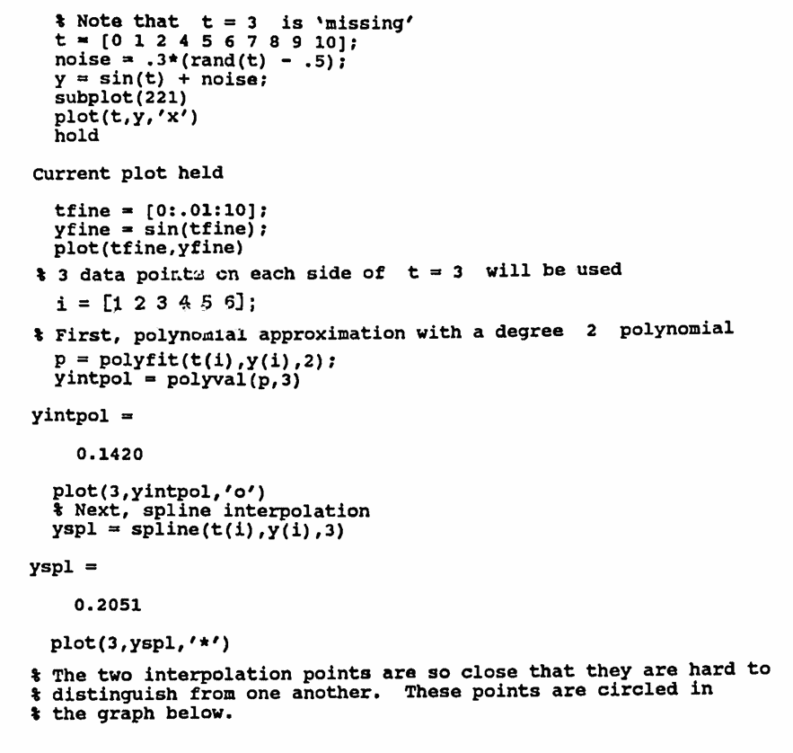
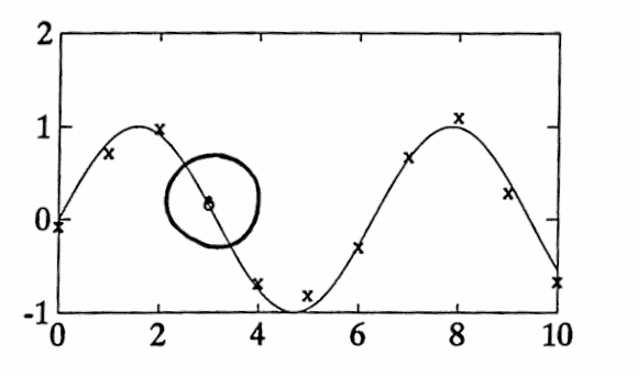
The following diary of an actual MATLAB session illustrates the use of the MATLAB commands discussed here.

A noisy data set, with a missing value, is generated. Both the  polyfit  and  spline  commands are used to fill in the missing value.

The MATLAB function given next computes the natural cubic spline. An example illustrating its similarity to the ‘not-a-knot’ spline follows.

Example

  t = [0:10];
  y = sin(t);
  subplot(221) % optional
  plot(t,y,'x')
  hold on

Current plot held

  tfine = [0:.1:10];
  yspl = spline(t,y,tfine);
  plot(tfine,yspl)
  natspl = cfspline(t,y,tfine);   plot(tfine,natspl,'.')

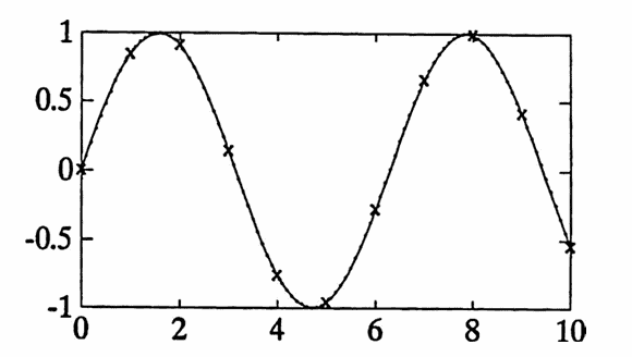
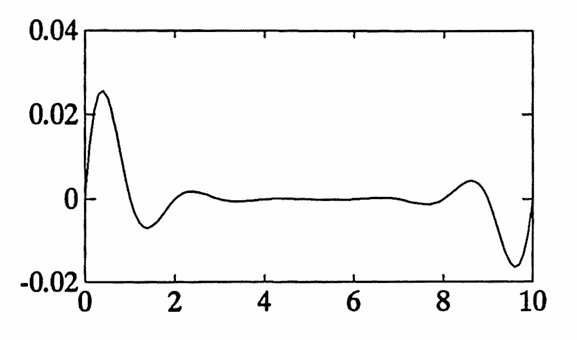
  % The two curves are so close that they are hard to distinguish.
  % The 'difference curve' is plotted next.
  hold off

Current plot released

  diff = yspl - natspl;
  plot(tfine,diff)