1.7 Historical Contributions in the Search for Hidden Periodicities

The purpose of this section is to highlight the historical developments in the search for hidden periodicities.

In so doing, it provides a gentle introduction to some important ideas that will discussed in greater detail throughout the dissertation. The presentation is chronological.

The Debut of the Sine Function

The ‘triangle’ approach to trigonometry appeared long before the emergence of the sine as a function of a continuous variable.

In about 160 B.C. the Greek astronomer Hipparchus investigated the complete measurement of triangles from certain data. Originally, one spoke not of the sine of an angle but instead of the sine of an arc, as follows.

Consider the circle below, with center $\,O\,$ and arc $\,AB\,.$ The length of the line segment $\,AM\,$ was defined to be the sine of the arc $\,AB\,$ [New, 18].

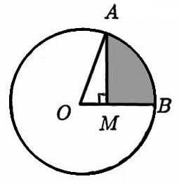
Why the word ‘sine’? Observe that the shaded shape resembles a stretched bow; indeed, the word sine derives from the Latin sinus, which means a bend [Oxf].

The word cosine uses the Latin prefix ‘co’, meaning in the company with, so that ‘cosine’ means in the company with the sine.

The view of sine and cosine as functions of a continuous variable is more advanced; it requires the use of a coordinate system to determine the appropriate signs (plus or minus) of the trigonometric functions for angles greater than ninety degrees.

This tool was not available until René Descartes (1596–1650) introduced what is now called the Cartesian coordinate system. With this graphical device, the center of the circle described above could be placed at the origin of the coordinate system, with segment $\,OB\,$ along the $x$-axis (see below).

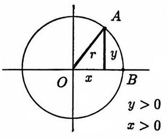
The ratio $\,\frac{\text{length of arc $AB$}}{\text{length of $OA$}}\,$ was known to be invariant under circle size, and is now known as the radian measurement of the angle. Call this ratio $\,u\,.$

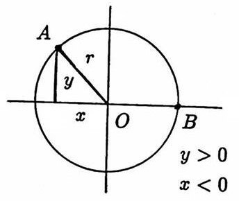
Then, the ratios $\,\frac{\text{length of $AM$}}{\text{length of $OA$}} := \frac yr\,$ and $\,\frac{\text{length of $OM$}}{\text{length of $OA$}} := \frac xr\,$ were defined as the sine of $\,u\,$ and cosine of $\,u\,,$ respectively, and these definitions could be preserved by paying attention to the signs of $\,x\,$ and $\,y\,$ in the various quadrants.

Thus, sine and cosine became separated from a study of triangles; the trigonometric functions had emerged [New, 39].

1500s–1600s: Interest in Naturally-Occurring Periodic Phenomena

During the 16^th and 17^th centuries, investigations into many naturally occurring physical problems helped to forward the interest in periodicity.

Johannes Kepler (1571–1630) derived the three basic laws of planetary motion that bear his name; for example, his law of periods states that the square of the period of a planet’s orbit about the sun is proportional to the cube of the planet’s mean distance from the sun [H&R, 262].

Galileo (1564–1642) observed that the periodic oscillation of a pendulum was independent of the mass of the suspended weight. Issac Newton (1642–1727) explained sound in terms of periodic waves [New, 412].

But the basis for modern theories of periodicity was to come in the 1700s, with the development of Fourier series.

1700s: Developments Due to a Vibrating String

Fourier analysis, which involves the representation of a function as a sum of sinusoids, is fundamental to many modern methods concerned with detecting hidden periodicities.

Thus, early developments by Jean LeRond d’Alembert (1707–1783), Leonhard Euler (1707–1783), Daniel Bernoulli (1700–1782), Joseph Louis Lagrange (1736–1813), and Jean-Baptiste-Joseph Fourier (1768–1830) are important.

This period of time is well documented, and the interested reader is referred to [Jef], [Car, 1–19], and [Gon, 427–441] for additional information.

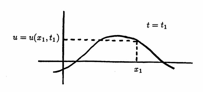
It was interest in the partial differential equation (PDE) now known as the one-dimensional homogeneous wave equation,

that led to the first investigations into the trigonometric expansion of a function. A solution $\,u(x,t)\,$ of this PDE gives the displacement of a particle at distance $\,x\,$ on a vibrating string at time $\,t\,.$

In 1746, the French mathematician d’Alembert obtained the solution

for an infinite length string, with zero initial vertical velocity and initial configuration $\,u(x,0) = f(x)\,.$ The constant $\,c\,$ depends on the string material.

This solution was arrived at by a change of variables, and required no trigonometric series results. Thus, existence of a solution (at least in the infinite length case) was established; the controversy that waged over the next couple decades concerned the form of the solution.

In 1753, Bernoulli [Ber, 173] claimed that the solution $\,u(x,t)\,$ for a finite string of length $\,\ell\,$ is expressible in the form:

This is the form obtained when one pursues the modern ‘separation of variables’ technique. When $\,t = 0\,,$ this reduces to an expression for the initial string displacement in the form:

Bernoulli believed that any initial displacement could be written in this way. Euler and d’Alembert disagreed: they argued that since sums of sine functions are both periodic and odd, any function which did not possess both these properties could not be expanded in such a way.

Thus began the animated debate over the representation of a function as a sum of sinusoids.

In 1777, Euler showed that if a function $\,f(x)\,$ could be represented in the form

then the coefficients must be given by:

However, it was Fourier, in his investigations of the PDE modeling the temperature distribution in a metal plate, who first applied these integral formulas to the representation of a completely arbitrary function.

In particular, Fourier allowed the function to have different analytical expressions in different parts of the interval. Also, he was the first to recognize that the use of sine series was not restricted to odd functions; and the use of cosine series was not restricted to even functions.

Further work by Cauchy (1789–1857), Dirichlet (1805–1859), Weierstrass (1815–1897), Riemann (1826–1866), Jordan (1838–1922), Cantor (1845–1918), and Lebesgue (1875–1941) passed into the realm of the pure mathematician.

These people made precise the notions of convergence, uniform convergence, functions, and integration which had been somewhat loose in earlier work, and thus laid the foundation for all modern analysis.

Backing up a bit in time, one of the first methods for detecting hidden periodicities was used by Lagrange in 1772 to analyze the orbit of a comet [Lag]. Lagrange had a good deal of interest in rational functions; one may recall the Lagrange Interpolation Formula

for the unique polynomial passing through $\,n + 1\,$ distinct data points $\,(x_i,f_i)_{i=0}^n\,.$ Thus it should not be surprising that Lagrange’s method used rational functions to analyze the data. Lagrange’s method was improved by Dale [Dale, 628] in 1778.

The next major contributions appeared in the mid 1800s, and are discussed in some detail in the following two sections.

1850–1900: Tabular Methods for Detecting Hidden Periodicities

In 1847, Buys-Ballot introduced a tabular method for detecting hidden periodicities that was used in his analysis of temperature variations [B-B, 34]. These methods were further developed by Strachey in 1877 [Str] and Stewart and Dodgson in 1878 [S&D].

The next example illustrates the ‘flavor’ of these tabular methods; note the similarity to the reshaping techniques discussed in Section 1.3. For more details, the reader is referred to [W&R, 345–362].

The scatter plot in Figure 1a (below) shows sixty unit-spaced data points; consecutive points have been connected by line segments in Figure 1b. This data was generated by the function

thus, it is a sum of a period $\,5\,$ sine curve of amplitude $\,2\,,$ a period $\,13\,$ cosine curve of amplitude $\,1\,,$ and noise, generated by the uniform distribution on $\,[-0.2, 0.2]\,.$

Now that you are privy to the generator of the data, forget it. The question is: “With only the sixty data points at hand—is it possible to recover any information regarding sinusoidal components?”

Figure 1

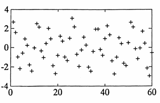
Figure 1a. A scatterplot of a function with two sinuosidal components, and noise.

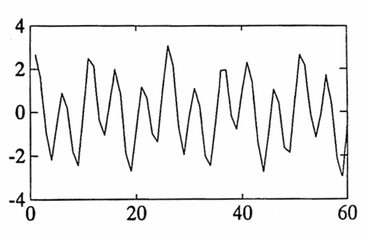
Figure 1b. The data in Figure 1a, with consecutive points connected by line segments.

The approach taken is roughly as follows: for a given period $\,p\,,$ get a number that reflects ‘how much’ this period is present in the data. Repeat the procedure for lots of values of $\,p\,$ and plot the results. The graph should peak at periodicities that are present in the data.

For example, let us test the data of Figure $1$ for period $\,5\,.$ Let $\,(i,y_i)\,$ denote the $\,i^{\text{th}}\,$ data point. First the data $\,\{y_1,y_2,y_3,\ldots,y_{60}\}\,$ must be arranged into rows of $\,5\,$; there will be $\,60/5\,$ such rows, as shown.

Next, sum the entries in each column and divide by the number of rows, thus obtaining the average value of each column. Let $\,M_i\,$ denote the average of the $\,i^{\text{th}}\,$ column. For the data above, we obtain the five numbers:

Finally, the standard deviation of the $\,M_i\,,$

is the number used to indicate ‘how much’ of period $\,5\,$ is present in the data. Of course, a reasonable question at this point is: Why this number?

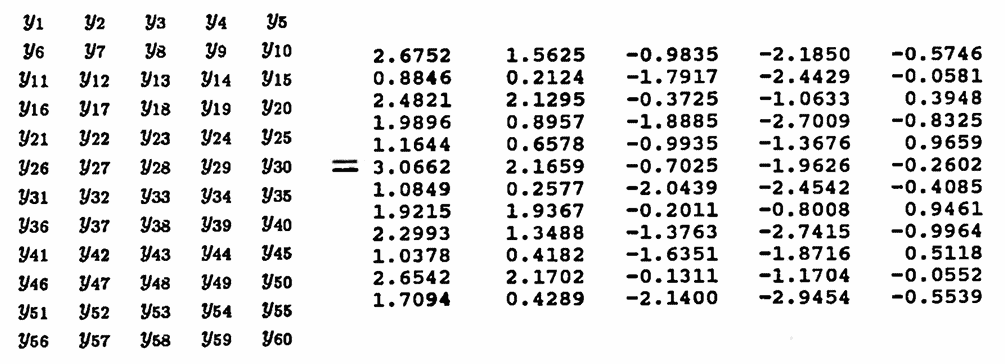
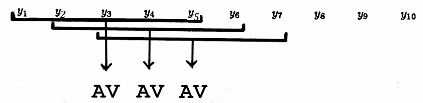
Here’s the rationale: Assume that the data is composed of sinusoidal components and random noise. If there is a component of period $\,5\,,$ then each column will contain the same phase of this component, as Figure 2a illustrates.

Figure 2a. Three components: period $\,5\,,$ period $\,13\,,$ and noise. All ‘dotted’ points will contribute to the same column in a tabular test for period $\,5\,.$

Averaging the column gives the correct amplitude of this component. But what of the other components—periodicities other than $\,5\,,$ and noise?

Since positive and negative deviations will tend to cancel each other, the averaging process will tend to annul these other components. So, the numbers $\,M_1\,$ through $\,M_5\,$ should be, approximately, as shown in Figure 2b (which they are!), and the standard deviation measures the spread of these values about their mean. Of course, the larger the amplitude of the component, the larger the spread about the mean.

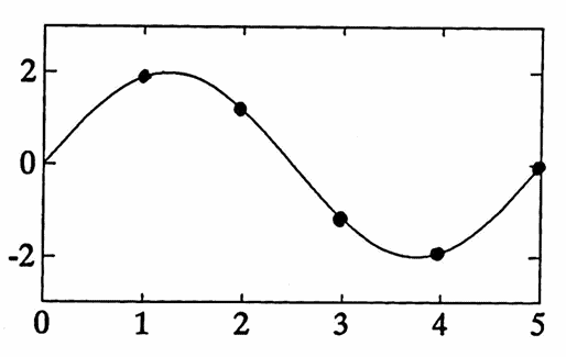
Figure 2b

Figure 3 shows the results of this test for periods up to $\,20\,.$ Indeed, a peak occurs at $\,5\,$ (and multiples of $\,5\,$). There is also a peak at $\,13\,,$ albeit less noticeable; partly because the amplitude of the cosine component is only half that of the sine component.

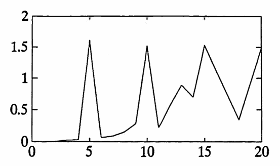
Figure 3. The ‘period detector number’ versus period. Note the peaks at $\,5\,$ (and multiples of $\,5\,$) and $\,13\,.$

About the same time that this tabular method was being pursued, Stokes [Sto] presented an integral approach to the problem. In 1879, he suggested that to test a function $\,f(x)\,$ for period $\,\frac{2\pi}n\,,$ one might do well to multiply by a sinusoid with this period, $\,\sin nx\,,$ and then investigate the integral:

For if $\,f(x)\,$ has a component $\,A\sin (n' x)\,,$ then this integral will involve (among other things):

The important observation is that if $\,n'\,$ is close to $\,n\,,$ then the sinusoid $\,\frac{A\sin\bigl((n'-n)x\bigr)}{2(n'-n)}\,$ has an amplitude of large magnitude and a long period, and should be easily detectable.

For example, taking $\,A = 1\,,$ $\,n' = 0.65\,$ and $\,n = 0.60\,$ yields the sine curve of amplitude $\,\frac 1{2(0.05)} = 10\,$ shown below:

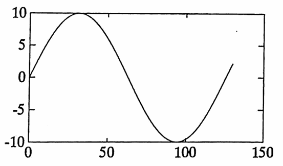
The graph of the sinusoid

when $\,A = 1\,,$ $\,n' = 0.65\,$ and $\,n = 0.60\,.$

1897: Schuster’s Periodogram

In 1897, Schuster introduced the periodogram as a tool for detecting hidden periodicities [Sch], and he used it to investigate meteorological phenomena. The method is computationally intensive, which made it difficult to apply practically until the advent of the electronic digital computer in 1946. A brief description and example follows.

Suppose there are $\,N\,$ available data points $\,(1,y_1),\ldots,(N,y_N)\,.$ Consider an approximation to the data of the form:

It is desired to choose the $\,2K+1\,$ coefficients $\,a_0,a_1,b_1,\ldots,a_K,b_K\,$ so that a least-squares fit is obtained. Provided that $\,N \ge 2K + 1\,,$ there is a unique solution to this problem, found by taking:

This is the discrete analogue of the (continuous) Fourier series, and is called the ‘discrete Fourier series corresponding to the data’ [S&H, 18–22].

Note that the fundamental frequency is $\,\frac 1N\,$; let $\,f_i := \frac iN\,$ denote the $\,i^{\text{th}}\,$ harmonic. The intensity at frequency $\,f_i\,$ is defined by $\,I(f_i)\,,$ where:

This intensity is measuring how much of the frequency $\,f_i\,$ is present in the data. The periodogram is the graph of $\,I(f_i)\,$ versus $\,f_i\,.$

To illustrate, consider again the data of Figure 1. Figure 5a (below) shows this data, superimposed with its discrete Fourier series.

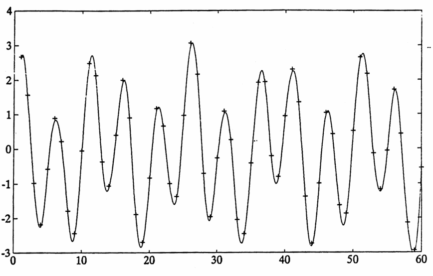
Figure 5a. A function having $\,2\,$ sinusoidal components and noise, superimposed with its discrete Fourier series.

Since $\,N\,$ is $\,60\,$ in this example, $\,K\,$ was taken to be $\,29\,,$ so that $\,K\,$ is the largest integer satisfying $\,2\cdot K + 1 \le 60\,.$

Figure 5b (below) shows the periodogram, which indeed peaks at both $\,f = 0.2\,$ and $\,f \approx 0.08\,$ (corresponding to periods $\,1/0.2 = 5\,$ and $\,1/0.08 = 12.5\,$).

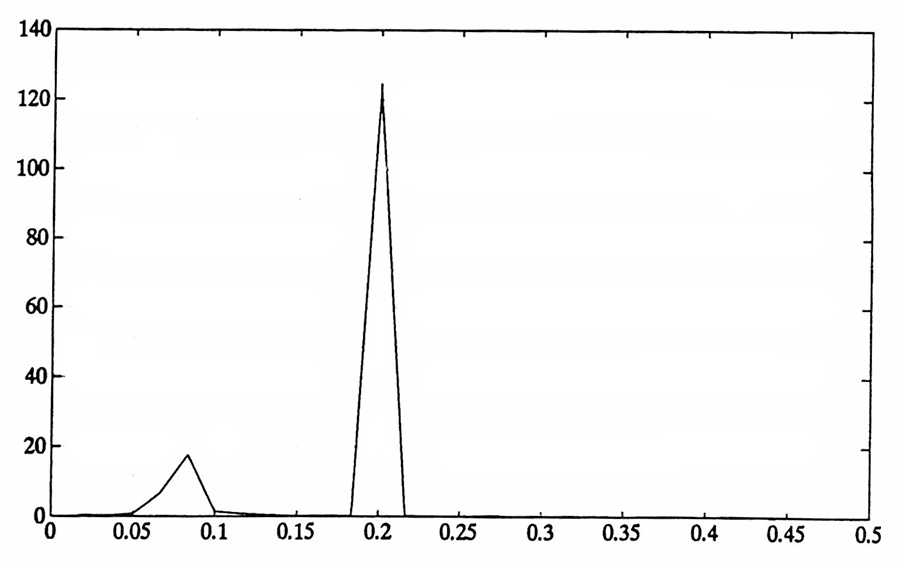
Figure 5b. The periodogram corresponding to the data in Figure 5a. Note the peaks, which detect the two sinusoidal components present in the data.

1900s: Time Series Analysis

The area of time series analysis really emerged—at least by this name—in the twentieth century. A time series is just an ordered list of numerical observations; this ‘ordering’ is usually provided by time, and hence the label.

Up until about 1925, a time series was analyzed as if it was deterministic: that is, a ‘generator’ (function of time) was sought that could subsequently be used to ‘determine’ values of the series. If the predicted values did not agree with the series values, blame was placed on an improper determination of the generator, or noise.

In 1927, an important new viewpoint emerged, due primarily to work on sunspot numbers by Udny Yule. He was struck by the ‘apparent’ periodicity of the data, speckled by irregularities, and drew this analogy:

If we have a rigid pendulum swinging under gravity through a small arc, its motion is well known to be harmonic, that is to say, it can be represented by a sine or cosine wave, and the amplitudes are constant, as are the periods of the swing.

But if a small boy now pelts the pendulum irregularly with peas the motion is disturbed. The pendulum will swing, but with irregular amplitudes and irregular intervals. The peas, in fact, instead of leading to behaviour in which any difference between theory and observation is attributable to an evanescent error, provide a series of shocks which are incorporated into the future motion of the system [Ken, 4].

From this viewpoint was to come the notion of a stochastic process, an important sub-area of time series analysis.

The probabilistic and statistical theory of time series was developed during the 1920s and 1930s, and the concept of spectrum was introduced [Blo, 6]. Roughly speaking, spectrum analysis is used to mean methods that describe the tendency for oscillations of a given frequency to appear in the data, rather than the oscillations themselves [Blo, 2]; spectrum analysis combines the methods of Fourier analysis and statistics.

The increased availability of computers in the 1950s and 1960s to carry out the extensive computations involved in spectrum analysis contributed to a wealth of developments in this decade: some important names are Grenander And Rosenblatt [G&R, 537–558], Parzen [Par], and Blackman and Tukey [B&T].

Signal Analysis

Parallel to the development of time series analysis is signal analysis. An important sub-area of signal analysis is filter theory—a filter being a device that transforms input in some specified way to yield a desired output [Joh, 1–3].

Filter theory began in 1915 when G.A. Campbell in America and Wagner in Germany independently invented the electric wave filter, a physical device to pass signals in a certain frequency band and suppress signals in all other bands. By providing different filters for different frequency ranges, more than one telephone conversation can be carried out simultaneously on the same lines [Mab, 31].

It is interesting to note that in early filter theory literature, the word ‘filter’ usually referred to the actual hardware—resistors, capacitors, inductors, and such—providing the signal processing. It was not until the 1930s (and the advent of so-called ‘modern filter theory’) that developments by Cauer, Darlington and others led to the idea of a mathematical filter and its associated transfer function, which describes precisely what the filter does.

As an example, consider the five-point moving average filter which takes five consecutive data points as input, averages them, and outputs the average, centered, as illustrated below.

By letting $\,a_n\,$ denote the average of data values $\,y_{n-2},\, y_{n-1},\, y_n,\, y_{n+1},\, y_{n+2}\,$ this filter can be described mathematically by:

The transfer function then describes what the filter does to each input frequency, as follows: notation is simplified tremendously if we work with the complex exponential

instead of real sines and cosines.

Suppose we ‘input’ a complex exponential of frequency $\,\omega\,,$

into the moving average filter $\,(\dagger)\,.$ Here, function notation $\,y(n)\,$ has been used instead of subscript notation $\,y_n\,,$ for convenience. The output obtained is:

The symmetry in the coefficients allowed use of the identity

to simplify the expression. If one defines

then it is seen that whenever $\,e^{i\omega n}\,$ is input to the filter, the corresponding output is $\,H(\omega)e^{i\omega n}\,.$ The critical observation is that the same function $\,e^{i\omega n}\,$ emerges from the filter , except multiplied by $\,H(\omega)\,.$

In practice, it is usually more convenient to work with cyclic frequency $\,f\,$ than radian frequency $\,\omega\,$; these are related by $\,\omega := 2\pi f\,.$ In terms of $\,f\,,$ the transfer function can be rewritten as:

This transfer function $\,\tilde H: f\mapsto \tilde H(f)\,$ is shown in Figure 6a (below) [Ham, 39]. Let’s reiterate how it works: if a sinusoidal component $\,S(t)\,$ of frequency $\,\tilde f\,$ is processed with this filter, the output will be $\,\tilde H(\tilde f)\cdot S(t)\,.$ That is, the transfer function $\,\tilde H\,$ allows one to take an input frequency $\,\tilde f\,$ and ‘transfer’ to the output simply by multiplying by $\,\tilde H(\tilde f)\,.$

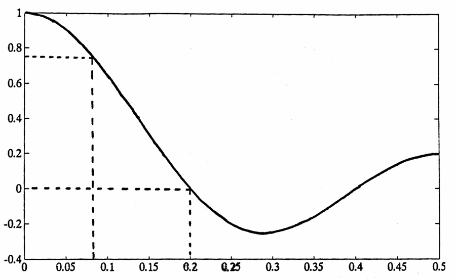
Figure 6a. The transfer function for a five-point moving average filter, $\tilde H(f)\,$ versus frequency $\,f\,.$ Note that $\tilde H(0.2) = 0\,$; a frequency $\,0.2\,$ (period $\,5\,$) sinusoid is completely suppressed.

Observe that the transfer function of Figure 6a has a zero at $\,f = 0.2\,,$ corresponding to period $\,5\,.$ Of course—if $\,5\,$ consecutive unit-spaced points are averaged on a period $\,5\,$ sinusoid, the result is zero! But if this filter acts on a sinusoid of period $\,13\,$ ($\,f = 1/13 \approx 0.08\,$), this component should emerge at approximately $\,0.7\,$ times its original amplitude.

To illustrate, this five-point moving average filter was applied to the sample data considered twice earlier; recall it has an amplitude $\,2\,$ component of period $\,5\,,$ an amplitude $\,1\,$ component of period $\,13\,,$ and some noise. The filter output is shown in Figure 6b (below). As expected, the period $\,5\,$ component has been entirely erased; all that remains is $\,0.7\,$ times the amplitude $\,1\,$ component!

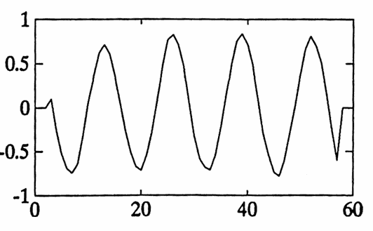
Figure 6b. The data of Figure 1a was filtered with a $5$-point moving average filter, yielding this output. Observe that only the period-$13$ component remains, at $\,0.7\,$ times its original amplitude.

Recent Developments

Often, the characteristics of a signal vary with time; for example, a ‘sinusoid’ may be present, but with period gradually increasing from $\,5\,$ to $\,7\,.$ A filter that tries to adapt to such changes is known as an adaptive filter. That is, the performance of the filter suggests changes in its coefficients [Ham, 277–278].

In 1960, R.E. Kalman introduced an algorithm since known as the discrete Kalman filter which is the main tool for such problems. His paper, titled A new approach to linear filtering and prediction problems, was published in the Journal of Basic Engineering, and is considered by many to be one of the most important results in its area in the last thirty years.

From a mathematical viewpoint, the Kalman filter theorem is a beautiful application of functional analysis; for statistics students, an example of Bayesian statistics in action [Cat, Preface & p. 137].

In 1965, Cooley and Tukey [C&T, 297–301] introduced an algorithm since known as a fast Fourier transform. Coupled with the smaller, faster and less expensive computers that appeared in the 1970s, many practical applications of spectrum analysis on large data sets became possible.

Techniques and methods that take advantage of increased computing powers will undoubtedly continue to advance the ‘search for hidden periodicities’.