Chapter 1: Periodic Functions
The purpose of computing is insight,
not numbers.
— R.W. Hamming
1.1 The Purpose of This Dissertation
This introductory section gives an informal discussion of the purpose of this dissertation. For this section only, the reader is assumed to have an intuitive understanding of the meaning of familiar words (like data set and periodic); precise meaning will be assigned to these concepts in later sections.
This dissertation is written for the person (hereafter called the analyst), who has a data set in hand, like
| $t$ | $y$ |
| 0 | 33.9300 |
| 2.0000 | 33.5100 |
| 4.0000 | 35.2900 |
| 6.0000 | 35.3900 |
| 8.0000 | 35.0100 |
| 10.0000 | 36.1700 |
| 12.0000 | 36.1100 |
| 14.0000 | 32.0300 |
| 16.0000 | 34.1200 |
| 18.0000 | 36.9200 |
| 20.0000 | 37.3400 |
| 22.0000 | 37.7600 |
| $\boldsymbol\vdots$ | $\boldsymbol\vdots$ |
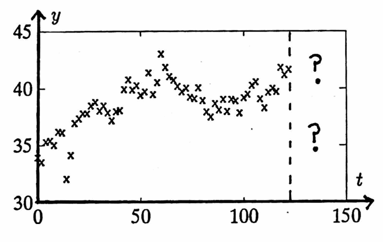
and who seeks to understand this data, for the primary purpose of predicting (forecasting) future behavior of the process that generated the data.
Such a data set is completely described by a finite collection of ordered pairs $\{(t_i,y_i)\ |\ i=1,\ldots,N\}\,.$ For most analysts, these ordered pairs will be stored in a computer in two columns (lists): a list of ‘input’ values $\,\{t_i\}_{i=1}^N\,$ and a list of corresponding ‘output’ values $\,\{y_i\}_{i=1}^N\,$:
| $t_1$ | $y_1$ |
| $t_2$ | $y_2$ |
| $t_3$ | $y_3$ |
| $\ \vdots$ | $\ \vdots$ |
| $t_N$ | $y_N$ |
The letter ‘$\,t\,$’ is used merely because time is a common input; and the letter ‘$\,y\,$’ is deeply entrenched in mathematical notation as denoting output values.
Different hypotheses (i.e., assumed truths) by the analyst regarding the nature of the data will lead to different methods for analyzing the data.
For example, based on experience or initial knowledge about the mechanism(s) generating the data, a researcher might be led to the hypothesis that a particular data set is a random walk [Dghty, 140–142]; or is a realization of a certain type of stochastic process [B&J]. Such hypotheses would dictate a particular investigative approach to be followed by the analyst.
The hypothesis to be investigated in this dissertation is that the output list is a finite sum of component functions. Particular emphasis is placed on the situation where at least one component is periodic. This type of hypothesis is investigated in the next example.
Example: The Output is a Finite Sum of Component Functions
Consider the schematic below, which illustrates two periodic components ($\,P_1\,$ has period $\,3\,,$ $\,P_2\,$ has period $\,7\,$) and a non-periodic component (a linear trend, $\,T\,$) that, together with some noise ($\,N\,$), sum to yield the data outputs denoted by $\,Y\,.$ Denote this by:
$$P_1 + P_2 + T + N = Y$$
Although, in this example, the components of $\,Y\,$ are known (they are $\,P_1\,,$ $\,P_2\,,$ $\,T\,,$ and $\,N\,$), one must remember that in actuality the analyst only has access to the data outputs $\,Y\,.$ Based on $\,Y\,$ alone, the analyst's hope is to recover information about the components, and then use this information to predict future values of $\,Y\,.$
It should be noted immediately that the components $\,P_1\,,$ $\,P_2\,,$ $\,T\,$ and $\,N\,$ are not unique; for example, any real number $\,K\,$ can be used to write $\,Y\,$ as a sum of four components:
$$ \overbrace{(P_1 - K)}^{\text{component $1$}} + \overbrace{(P_2 + K)}^{\text{component $2$}} + T + N = Y $$The ‘new’ component $\,P_1 - K\,$ still has period $\,3\,$; the ‘new’ component $\,P_2 + K\,$ still has period $\,7\,$; and these four components still sum to give $\,Y\,.$ Many other combinations are possible. Thus, there is no hope of recovering the exact components that make up the output data.
The output list $\,Y\,$ just constructed is an example of what will be referred to, throughout this dissertation, as a known unknown. It is known because it was constructed by the analyst. However, the components that make up $\,Y\,$ will be assumed to be unknown (to varying degrees) in order to test various techniques for identifying components.
A very simple example is presented next to illustrate some important logical considerations that must constantly be kept in mind. Suppose that an analyst is presented with the (unrealistically small) data set:
$$ \begin{align} (t_1,y_1) &= (\ \ T,1)\cr (t_2,y_2) &= (2T,2)\cr (t_3,y_3) &= (3T,3)\cr (t_4,y_4) &= (4T,4)\cr \end{align} $$This data is stored in the computer as two columns of numbers:
| $\ \ T$ | $1$ |
| $2T$ | $2$ |
| $3T$ | $3$ |
| $4T$ | $4$ |
Here, $\,T\,$ is any positive number; the particular value of $\,T\,$ is unimportant to the current discussion, except for the consequence that the data is equally-spaced. This data set is graphed below.
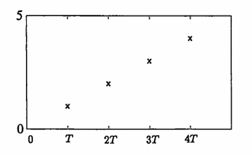
Unknown to the analyst, this data was generated as the sum of a $2$-cycle and a $3$-cycle,
$$ \begin{align} &(\ \ \ 3,\ \ \ \ 6,\ \ 3,\ \ \ \, 6,\ \ \ \, 3,\ \ 6,\ \ \ \ 3,\ \ \ \, 6,\ \ 3,\, \ldots)\cr +\ \ &({-}2,\, {-}4,\ \ 0,\, {-}2,\, {-}4,\ \ 0,\, -2,\, {-}4,\ \ 0,\, \ldots)\cr =\ &(\ \ \ 1,\ \ \ \ 2,\ \ 3,\ \ \ \ 4,\, -1,\ \ 6,\ \ \ \, 1,\ \ \ \ 2,\ \ 3,\, \ldots)\,, \end{align} $$producing a $6$-cycle; but not even one cycle of the resulting $6$-cycle has yet been observed by the analyst. Now that you are privy to this component information, forget it, and continue with the analysis.
Based on the four pieces of observed data $\,(1,2,3,4)\,,$ you, as the analyst, hope to predict future behavior. Thus, you make an initial hypothesis:
HYPOTHESIS #1: The data is being generated by the linear function $\,y_n = n\,.$
Based on this hypothesis, you predict the next data point:
$$(y_5)_{\text{predicted}} = 5$$When the next data value, $\,-1\,,$ becomes available, you have learned something: your hypothesis, at least in its ‘purest’ form, was incorrect.
Let’s look at the logic underlying this conclusion. Remember that the mathematical sentence
$$\text{‘If $\,A\,,$ then $\,B\,$’}\tag{S1}$$is logically equivalent to its contrapositive,
$$\text{‘If not $\,B\,,$ then not $\,A\,$’}\tag{S2}$$For ease of notation, denote the sentence ‘If $\,A\,,$ then $\,B\,$’ by S1; and denote the sentence ‘If not $\,B\,,$ then not $\,A\,$’ by S2.
The fact that S1 is logically equivalent to S2 means that S1 and S2 always have the same truth values: if S1 is true, so is S2; if S1 is false, so is S2; if S2 is true, so is S1; and if S2 is false, so is S1. (See Appendix 1 for a discussion of mathematical logic.)
The sentence
IF the data set is generated by $\,y_n = n\,,$ THEN $\,y_5 = 5$
is a true mathematical sentence. Therefore, its contrapositive,
IF $\,y_5 \ne 5\,,$ THEN the data set is not generated by $\,y_n = n$
is also true. Since $\,y_5 \ne 5\,$ (is true), it is concluded that $\,y_n = n\,$ is not the correct generator for the data.
Since hypothesis #1 is incorrect, it is discarded, and a new hypothesis is sought. The analyst is still struck by the linearity of the first four data values, and decides that this fifth data value is an anomaly—a mistake—an outlier—caused perhaps by some temporary outside influence. Thus, the hypothesis is only slightly modified:
HYPOTHESIS #2: The data set is being generated by the function $\,y_n = n\,,$ for all $\,n \ne 5\,.$
Under this slightly modified hypothesis, the next data value is predicted: $\,(y_6)_{\text{predicted}} = 6\,.$ When the next data value is observed, one indeed sees that $\,y_6 = 6\,.$
This new information supports hypothesis #2. That is, at this point, there is no reason to reject hypothesis #2. However, the analyst cannot conclude that hypothesis #2 is true. It might be (as, indeed it is) that $\,y_6\,$ equals $\,6\,$ for reasons other than hypothesis #2 being true.
Keeping hypothesis #2, the analyst predicts that $(y_7)_{\text{predicted}} = 7\,.$ Upon observing $\,y_7 = 1\,,$ however, hypothesis #2 must be discarded.
Suppose that the analyst is fortunate enough to make the following conjecture (educated guess):
HYPOTHESIS #3: The output list is a sum of a $2$-cycle and a $3$-cycle.
Such a sum must repeat itself every six entries. Consequently, if hypothesis #3 is made after having observed the first six outputs $\,(1,2,3,4,-1,6)\,,$ then no analysis needs to be done; the analyst immediately concludes that these six outputs must repeat themselves:
$$ (\overbrace{1,2,3,4,-1,6}^{\text{first six outputs ...}}, \overbrace{1,2,3,4,-1,6}^{\text{... repeat themselves}},\ldots) $$Although future values have been correctly predicted in this case, the analyst may still desire more information about the components making up the output list. Some basic reshaping techniques (discussed in section 1.3) can be used on the first six pieces of data to find two components that can be used for prediction. The technique is illustrated next:
- Let $\,\boldsymbol{\rm Y} = (1,2,3,4,—1,6)\,.$
-
Find the mean (average) of the entries in $\,\boldsymbol{\rm Y}\,,$ and denote it by $\,\mu_{\boldsymbol{\rm Y}}\,$:
$$ \begin{align} \mu_{\boldsymbol{\rm Y}} &= \frac 16(1 + 2 + 3 + 4 + (-1) + 6)\cr\cr &= 2.5 \end{align} $$ -
Construct a ‘mean-zero’ output list $\,\boldsymbol{\rm Y}_0\,$ by subtracting $\,\mu_{\boldsymbol{\rm Y}}\,$ from each entry in $\,\boldsymbol{\rm Y}\,$:
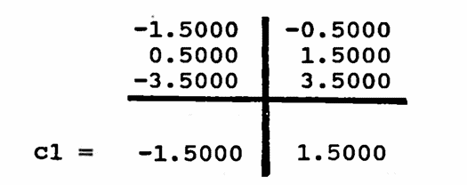
$$ \begin{align} \boldsymbol{\rm Y}_0 &=\ \ \ \, (\ \ \ \ \ \ \, 1,\ \ \ \ \ \, 2,\ \ \ \ \, 3,\ \ \ \, 4,\ \ \, {-}1,\ \ \ \ 6)\cr\cr &\quad - (\ \ \ \, 2.5,\ \ \ 2.5,\ 2.5,\ 2.5,\ \ \, 2.5,\ 2.5)\cr\cr &=\quad (-1.5, -0.5,\ 0.5,\ 1.5, -3.5,\ 3.5) \end{align} $$ -
‘Reshape’ $\,\boldsymbol{\rm Y}_0\,$ to test for a period-$2$ component, and take the mean of each column. This gives the mean-zero $2$-component, called cl below.
-
‘Reshape’ $\,\boldsymbol{\rm Y}_0\,$ to test for a period-$3$ component, and take the mean of each column. This gives the mean-zero $3$-component, called c2 below.

-
If $\,\boldsymbol{\rm Y}\,$ is indeed the sum of a $2$-cycle and a $3$-cycle, then adding $\,\mu_{\boldsymbol{\rm Y}}\,$ to c1 and c2 must give back $\,\boldsymbol{\rm Y}\,,$ and it does: $$ \begin{align} &(-1.5,\ 1.5,\ -1.5,\ 1.5,\ -1.5,\ 1.5)\cr\cr +\ &(\quad\ \ 0,\ \ {-}2,\qquad 2,\quad\, 0,\quad\ \ {-}2,\ \ \ \ 2)\cr\cr +\ &(\quad 2.5,\ \, 2.5,\ \ \ \ \, 2.5,\ \ 2.5,\ \ \ \ \ \, 2.5,\, 2.5)\cr\cr =\ &(\qquad 1,\ \ \ \, 2,\qquad 3,\quad\ 4,\quad\ \, {-}1,\ \ \ \ 6) \end{align} $$
It is interesting to note that if the output list is truly a sum of a $2$-cycle and a $3$-cycle, then once only $\,4\,$ outputs have been observed, future behavior can be predicted. See section 1.5 for details.
Example
Here is a second example, more realistic in terms of data set size than the first, which also emphasizes the problem of not knowing if a hypothesis is true.
Suppose that an analyst is presented with the data set shown below:
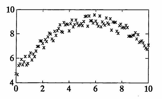
Unknown to the analyst, this data set was generated by the continuous function
$$ y(t) = 3\sin\bigl(\frac{2\pi t}{20}\bigr) + 0.2t + 5 + \langle\text{noise}\rangle\,, $$sampled at increments of $\,0.1\,$ on the interval $\,[0,10]\,.$
The data certainly looks like a piece of a parabola, and the analyst may make the initial hypothesis:
HYPOTHESIS #1: $\,h_1(t) = b_0 + b_1t + b_2t^2$
Motivated by this hypothesis, values of $\,b_0\,,$ $\,b_1\,,$ and $\,b_2\,$ are sought so that $\,h_1(t)\,$ ‘fits’ the data in the best least-squares sense (see section 2.2).
Having done so, the analyst finds that the agreement between $\,h_1(t)\,$ (the hypothesized data generator) and $\,y(t)\,$ (the actual data) looks beautiful on the original data interval $\,[0,10]\,.$ However, when $\,h_1(t)\,$ is used to forecast behavior on the interval $\,[10,15]\,,$ a comparison with $\,y(t)\,$ shows that the fit is terrible.
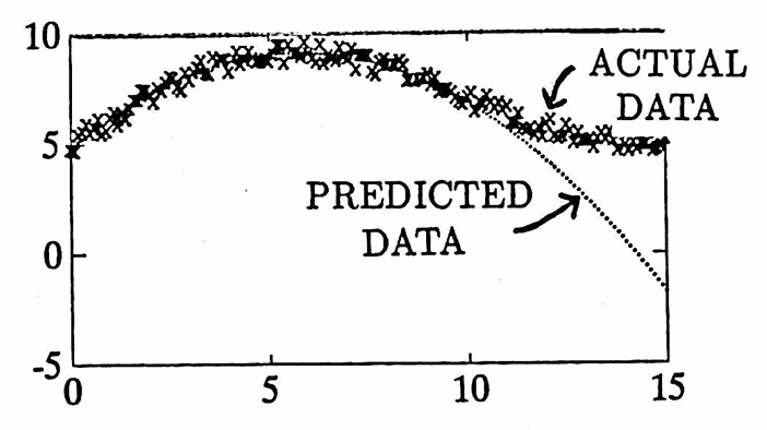
The hypothesized components led to a ‘fit’ that was beautiful on the data currently available to the analyst. However, using this ‘fit’ to predict future values led to huge errors. What happened?
It is indeed true that IF the hypothesis is correct, THEN the fit will be beautiful. However, the ‘fit’ may be beautiful for reasons other than the hypothesis being correct.
In this case, the Weierstrass Approximation Theorem [Bar, p. 172] can be cited as the reason that the ‘fit’ is beautiful. This theorem states that any continuous function defined on a closed interval can be uniformly approximated by polynomials; consequently, a good ‘fit’ can always be obtained, if a sufficiently high degree polynomial is used.
The moral is: A ‘beautiful fit’ never assures the analyst that the conjectured components are correct.
The fit may be beautiful for reasons other than the hypothesis being correct, potentially rendering the hypothesized components useless for predictive purposes.
R.W. Hamming, author of several books in numerical analysis and digital filters, emphasizes that the purpose of computing is insight, not numbers. The analyst must always be attentive to the possibility that the hypotheses are not correct.